Arrangements of Stars on the American Flag

Reasonable star patterns on the American flag correspond to special factorizations; the density of such factorizations is less than the density of values in a multiplication table; Paul Erdös showed this density asymptotically approaches zero by considering the average number of prime factors of an integer. – See more at: http://www.maa.org/programs/maa-awards/writing-awards/lester-r-ford-awards/arrangements-of-stars-on-the-american-flag#sthash.e9PHpilF.dpuf

Read the article here: http://www.maa.org/programs/maa-awards/writing-awards/lester-r-ford-awards/arrangements-of-stars-on-the-american-flag

US vs UK: Mathematical Terminology

Math With Bad Drawings had an amusing essay concerning differences in mathematical nomenclature between American English and British English. I thought that it would be appropriate to share this around the Fourth of July.

From the essay and the comments to the essay:

Math vs. maths
Zee vs. zed
$3.5$ vs. $3\cdot 5$
Trapezoid vs. trapezium
Scientific notation vs. standard form
Exponents vs. indices
Revise and review vs. review and revise
Imperial units vs. metric units
Pythagorean theorem vs. Pythagoras
Slope vs. gradient
Root vs. surd
PEMDAS vs. BIMDAS
Billion vs. trillion (a generation ago)
GCD (greatest common divisor) vs. HCF (highest common factor)

Proving theorems and special cases (Part 17): Conclusion

In a recent class with my future secondary math teachers, we had a fascinating discussion concerning how a teacher should respond to the following question from a student:

Is it ever possible to prove a statement or theorem by proving a special case of the statement or theorem?

Usually, the answer is no. In this series of posts, we’ve seen that a conjecture could be true for the first 40 cases or even the first $10^{316}$ cases yet not always be true. We’ve also explored the computational evidence for various unsolved problems in mathematics, noting that even this very strong computational evidence, by itself, does not provide a proof for all possible cases.

Source: http://mathwithbaddrawings.com/2015/06/24/mathemacomics/

However, there are plenty of examples in mathematics where it is possible to prove a theorem by first proving a special case of the theorem. As I’ve hopefully shown through this series, using only examples that could appear in the secondary curriculum, this is a technique that comes up again and again in mathematics, and here’s a story that a like to tell my students to get this idea across.

Here’s a story that I’ll tell my students when, for the first time in a semester, I’m about to use a lemma to make a major step in proving a theorem. (I think I was 13 when I first heard this one, and obviously it’s stuck with me over the years.)

At MIT, there’s a two-part entrance exam to determine who will be the engineers and who will be the mathematicians. For the first part of the exam, students are led one at a time into a kitchen. There’s an empty pot on the floor, a sink, and a stove. The assignment is to boil water. Everyone does exactly the same thing: they fill the pot with water, place it on the stove, and then turn the stove on. Everyone passes.

For the second part of the exam, students are led one at a time again into the kitchen. This time, there’s a pot full of water sitting on the stove. The assignment, once again, is to boil water. Nearly everyone simply turns on the stove. These students are led off to become engineers. The mathematicians are ones who take the pot off the stove, dump the water into the sink, and place the empty pot on the floor… thereby reducing to the original problem, which had already been solved.

Proving theorems and special cases (Part 16): An old homework problem

In a recent class with my future secondary math teachers, we had a fascinating discussion concerning how a teacher should respond to the following question from a student:

Is it ever possible to prove a statement or theorem by proving a special case of the statement or theorem?

However, there are plenty of examples in mathematics where it is possible to prove a theorem by first proving a special case of the theorem. For the remainder of this series, I’d like to list, in no particular order, some common theorems used in secondary mathematics which are typically proved by first proving a special case.

The following problem appeared on a homework assignment of mine about 30 years ago when I was taking Honors Calculus out of Apostol’s book. I still remember trying to prove this theorem (at the time, very unsuccessfully) like it was yesterday.

Theorem. If $f(x)$ is a continuous function so that $f(x+y) = f(x) + f(y)$ , then $f(x) = cx$ for some constant $c$ .

Proof. The proof mirrors that of the uniqueness of the logarithm function, slowly proving special cases to eventually prove the theorem for all real numbers $x$ .

Case 1. $x = 0$ . If we set $x =0$ and $y = 0$ , then

$f(0+0) = f(0) + f(0)$

$f(0) = 2 f(0)$

$0 = f(0)$

Case 2. $x \in \mathbb{N}$ . If $x$ is a positive integer, then

$f(x) = f(1 + 1 + \dots + 1)$

$f(x) = f(1) + f(1) + \dots + f(1)$

$f(x) = xf(1)$ .

(Technically, this should be proven by induction, but I’ll skip that for brevity.) If we let $c = f(1)$ , then $f(x) = cx$ .

Case 3. $x \in \mathbb{Z}$ . If $x$ is a negative integer, let $x = -n$ , where $n$ is a positive integer. Then

$f(x + (-x)) = f(x) + f(-x)$

$f(0) = f(x) + f(n)$

$0 = f(x) + cn$

$-cn = f(x)$

$cx = f(x)$

Case 4. $x \in \mathbb{Q}$ . If $x$ is a rational number, then write $x = p/q$ , where $p$ and $q$ are integers and $q$ is a positive integer. We’ll use the fact that $p = xq = p/q \times q = p/q + p/q + \dots + p/q$ , where the sum is repeated $q$ times.

$f(p/q + p/q + \dots + p/q) = f(p)$

$f(p/q) + f(p/q) + \dots + f(p/q) = cp$

$q f(p/q) = cp$

$f(p/q) = cp/q$

$f(x) = cx$

Case 5. $x \in \mathbb{R}$ . If $x$ is a real number, then let $\{r_n\}$ be a sequence of rational numbers that converges to $x$ , so that

$\lim_{n \to \infty} r_n = x$

Then, since $f$ is continuous,

$f(x) = f \left( \displaystyle \lim_{n \to \infty} r_n \right)$

$f(x) =\displaystyle \lim_{n \to \infty} f(r_n)$

$f(x) = \displaystyle \lim_{n \to \infty} c r_n$

$f(x) = cx$

QED

Random Thought #1: The continuity of the function $f$ was only used in Case 5 of the above proof. I’m nearly certain that there’s a pathological discontinuous function that satisfies $f(x+y) = f(x) + f(y)$ which is not the function $f(x) = cx$ . However, I don’t know what that function might be.

Random Thought #2: For what it’s worth, this same idea can be used to solve the following problem that was posed during UNT’s Problem of the Month competition in January 2015. I won’t solve the problem here so that my readers can have the fun of trying to solve it for themselves.

Problem. Determine all nonnegative continuous functions that satisfy

$f(x+t) = f(x) + f(t) + 2 \sqrt{f(x)} \sqrt{f(t)}$ .

Proving theorems and special cases (Part 15): The Mean Value Theorem

In a recent class with my future secondary math teachers, we had a fascinating discussion concerning how a teacher should respond to the following question from a student:

Is it ever possible to prove a statement or theorem by proving a special case of the statement or theorem?

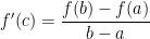
6. Theorem (Mean Value Theorem). If $f$ is a continuous function on the interval $[a,b]$ which is differentiable on the interior $(a,b)$ , then there is a point $c \in (a,b)$ so that

$f'(c) = \displaystyle \frac{f(b)-f(a)}{b-a}$

In other words, there is a point $c$ in $(a,b)$ so that the slope of the tangent line at $c$ is the same as the slope of the line segment connecting the endpoints.

This is a consequence of the following lemma.

Lemma (Rolle’s Theorem). If $f$ is a continuous function on the interval $[a,b]$ which is differentiable on the interior $(a,b)$ so that $f(a) = 0$ and $f(b) = 0$ , then there is a point $c \in (a,b)$ so that $f'(c) = 0$ .

Notice that Rolle’s Theorem is really a special case of the Mean Value Theorem: if $f(a) = 0$ and $f(b) = 0$ , then the right-hand side of the conclusion of the Mean Value Theorem becomes

$\displaystyle \frac{f(b)-f(a)}{b-a} = \displaystyle \frac{0-0}{b-a} = 0$ ,

thus matching the conclusion of Rolle’s Theorem.

I won’t type out the proofs of Rolle’s Theorem and the Mean Value Theorem here, since Wikipedia has already done that very well. Suffice it to say that Rolle’s Theorem logically comes first, and then the Mean Value Theorem can be proven using Rolle’s Theorem. The main idea is to assume that the function $f$ satisfies the hypotheses of the Mean Value Theorem and then define

$g(x) = f(x) - f(a) - \displaystyle \frac{f(b)-f(a)}{b-a} (x-a)$

It’s straightforward to show that $g$ satisfies the hypotheses of Rolle’s Theorem and conclude that there must be a point so that $g'(c) = 0$ , from which we obtain the conclusion of the Mean Value Theorem.

Proving theorems and special cases (Part 14): The Power Law of differentiation

In a recent class with my future secondary math teachers, we had a fascinating discussion concerning how a teacher should respond to the following question from a student:

Is it ever possible to prove a statement or theorem by proving a special case of the statement or theorem?

5. Theorem. For any rational number $r$ , we have $\displaystyle \frac{d}{dx} x^r = r x^{r-1}$ .

This theorem is typically proven using the Chain Rule (in the guise of implicit differentiation) and the following lemma:

Lemma. For any integer $n$ , we have $\displaystyle \frac{d}{dx} x^n = n x^{n-1}$ .

Clearly, the lemma is a special case of the main theorem. However, the lemma can be proven without using the main theorem:

Proof of Lemma (Case 1). If $n$ is a positive integer, then

$\displaystyle \frac{d}{dx} x^n = \displaystyle \lim_{h \to 0} \frac{(x+h)^n - x^n}{h}$

$= \displaystyle \lim_{h \to 0} \frac{x^n + n x^{n-1} h + \frac{1}{2} n(n-1) x^{n-2} + \dots + h^n - x^n}{h}$

$= \displaystyle \lim_{h \to 0} \left[ n x^{n-1} + \frac{1}{2} n(n-1) x^{n-2} h + \dots + h^{n-1} \right]$

$= n x^{n-1} + 0 + \dots + 0$

$= n x^{n-1}$

Case 1 can also be proven using the Product Rule and mathematical induction.

Proof of Lemma (Case 2). If $n = 0$ , then the theorem is trivially true since $x^0 = 1$ , and the derivative of a constant is zero.

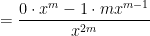
Proof of Lemma (Case 3). If $n$ is a negative integer, then write $n = -m$ , where $m$ is a positive integer. Then, using the Quotient Rule,

$\displaystyle \frac{d}{dx} x^n = \displaystyle \frac{d}{dx} \left( x^{-m} \right)$

$= \displaystyle \frac{d}{dx} \left( \frac{1}{x^m} \right)$

$= \displaystyle \frac{0 \cdot x^m - 1 \cdot m x^{m-1}}{x^{2m}}$

$= -m x^{-m - 1}$

$= n x^{n-1}$

QED

Now that the lemma has been proven, the main theorem can be proven using the lemma.

Proof of Theorem. Suppose that $r = p/q$ , where $p$ and $q$ are integers. Suppose that $y = x^r = x^{p/q}$ . Then:

$y = x^{p/q}$

$y^q = \displaystyle \left[ x^{p/q} \right]^q$

$y^q = x^p$

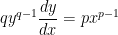
Let’s now differentiate with respect to $x$ :

$q y^{q-1} \displaystyle \frac{dy}{dx} = p x^{p-1}$

$\displaystyle \frac{dy}{dx} = \displaystyle \frac{p x^{p-1}}{q y^{q-1}}$

$\displaystyle \frac{dy}{dx} = \displaystyle \frac{p}{q} \frac{x^{p-1}}{[x^{p/q}]^{q-1}}$

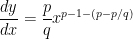
$\displaystyle \frac{dy}{dx} = \displaystyle \frac{p}{q} \frac{x^{p-1}}{x^{p - p/q}}$

$\displaystyle \frac{dy}{dx} = \displaystyle \frac{p}{q} x^{p-1 - (p-p/q)}$

$\displaystyle \frac{dy}{dx} = \displaystyle \frac{p}{q} x^{p - 1 - p + p/q}$

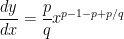
$\displaystyle \frac{dy}{dx} = \displaystyle \frac{p}{q} x^{p/q - 1}$

$\displaystyle \frac{dy}{dx} = r x^{r-1}$

QED

Proving theorems and special cases (Part 13): Uniqueness of logarithms

In a recent class with my future secondary math teachers, we had a fascinating discussion concerning how a teacher should respond to the following question from a student:

Is it ever possible to prove a statement or theorem by proving a special case of the statement or theorem?

The next theorem is needed in calculus to show that $\ln x = \displaystyle \int_1^x \frac{dt}{t}$ .

4. Theorem. Let $a \in \mathbb{R}^+ \setminus \{1\}$ . Suppose that $f: \mathbb{R}^+ \rightarrow \mathbb{R}$ has the following four properties:

$f(1) = 0$
$f(a) = 1$
$f(xy) = f(x) + f(y)$ for all $x, y \in \mathbb{R}^+$
$f$ is continuous

Then $f(x) = \log_a x$ for all $x \in \mathbb{R}^+$ .

In other blog posts, I went through the full proof of this theorem, which is divided — actually, scaffolded — into cases:

Case 1. $f(x) = \log_a x$ if $x$ is a positive integer.

Case 2. $f(x) = \log_a x$ if $x$ is a positive rational number.

Case 3. $f(x) = \log_a x$ if $x$ is a negative rational number.

Case 4. $f(x) = \log_a x$ if $x$ is a real number.

Clearly, Case 1 is a subset of Case 2, and Case 3 is a subset of Case 4. Once again, a special case of a theorem is used to prove the full theorem.

Proving theorems and special cases (Part 12): The sum and difference formulas for sine

In a recent class with my future secondary math teachers, we had a fascinating discussion concerning how a teacher should respond to the following question from a student:

Is it ever possible to prove a statement or theorem by proving a special case of the statement or theorem?

3. Theorem 1. $\sin(\alpha + \beta) = \sin \alpha \cos \beta + \cos \alpha + \sin \beta$

Theorem 2. $\sin(\alpha - \beta) = \sin \alpha \cos \beta - \cos \alpha \sin \beta$

For angles that are not acute, these theorems can be proven using a unit circle and the following four lemmas:

Lemma 1. $\cos(x - y) = \cos x \cos y + \sin x \sin y$

Lemma 2. $\cos(x + y) = \cos x \cos y - \sin x \sin y$

Lemma 3. $\sin(\pi/2 - x) = \cos x$

Lemma 4. $\cos(\pi/2 - x) = \sin x$

Specifically, assuming Lemmas 1-4, then:

$\sin(\alpha + \beta) = \cos(\pi/2 - [\alpha + \beta])$ by Lemma 4

$= \cos([\pi/2 - \alpha] - \beta)$

$= \cos(\pi/2 - \alpha) \cos \beta + \sin(\pi/2 - \alpha) \sin \beta$ by Lemma 1

$= \sin \alpha \cos \beta + \cos \alpha \sin \beta$ by Lemmas 3 and 4.

Also,

$\sin(\alpha - \beta) = \cos(\pi/2 - [\alpha - \beta])$ by Lemma 4

$= \cos([\pi/2 - \alpha] + \beta)$

$= \cos(\pi/2 - \alpha) \cos \beta - \sin(\pi/2 - \alpha) \sin \beta$ by Lemma 2

$= \sin \alpha \cos \beta - \cos \alpha \sin \beta$ by Lemmas 3 and 4.

However, we see that what I’ve called Lemma 3, often called a cofunction identity, can be considered a special case of Theorem 2. However, this is not circular logic since the cofunction identities can be proven without appealing to Theorems 1 and 2.

Proving theorems and special cases (Part 11): The Law of Cosines

In a recent class with my future secondary math teachers, we had a fascinating discussion concerning how a teacher should respond to the following question from a student:

Is it ever possible to prove a statement or theorem by proving a special case of the statement or theorem?

2. Theorem. In $\triangle ABC$ where $a = BC$ , $b = AC$ , and $c = AB$ , we have $c^2 = a^2 + b^2 - 2 a b \cos (m \angle C)$ .

This is typically proven using the Pythagorean theorem:

Lemma. In right triangle $\triangle ABC$ , where $\angle C$ is a right angle, we have $c^2 = a^2 + b^2$ .

Though it usually isn’t thought of this way, the Pythagorean theorem is a special case of the Law of Cosines since $\cos 90^\circ = 0$ .

There are well over 100 different proofs of the Pythagorean theorem that do not presuppose the Law of Cosines. The standard proof of the Law of Cosines then uses the Pythagorean theorem. In other words, a special case of the Law of Cosines is used to prove the Law of Cosines.

Proving theorems and special cases (Part 10): Angles in a convex n-gon

In a recent class with my future secondary math teachers, we had a fascinating discussion concerning how a teacher should respond to the following question from a student:

Is it ever possible to prove a statement or theorem by proving a special case of the statement or theorem?

1. Theorem. The sum of the angles in a convex n-gon is $180(n-2)$ degrees.

This theorem is typically proven after first proving the following lemma:

Lemma. The sum of the angles in a triangle is $180$ degrees.

Clearly the lemma is a special case of the main theorem: for a triangle, $n=3$ and so $180(n-2) = 180 \times 1 = 180$ . The proof of the lemma uses alternate interior angles and the convention that the angle of a straight line is 180 degrees.

Using this, the main theorem follows by using diagonals to divide a convex n-gon into $n-2$ triangles. (For example, drawing a diagonal divides a quadrilateral into two triangles.) The sum of the angles of the n-gon must equal the sum of the angles of the $n-2$ triangles.

So it is possible to prove a theorem by proving a special case of the theorem. Using the sum of the angles of a triangle to prove the formula for the sum of the angles of a convex n-gon is qualitatively different than the previous computational examples seen earlier in this series.