Thoughts on 1/7 and other rational numbers (Part 9)

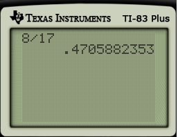
Let’s now consider the decimal representation of $\displaystyle \frac{8}{17}$ .

There’s no obvious repeating pattern. But we know that, since 17 has neither 2 nor 5 as a factor, that there has to be a repeating decimal pattern.

So… what is it?

When I ask this question to my students, I can see their stomachs churning a slow dance of death. They figure that the calculator didn’t give the answer, and so they have to settle for long division by hand.

That’s partially correct.

However, using the ideas presented below, we can perform the long division extracting multiple digits at once. Through clever use of the calculator, we can quickly obtain the full decimal representation even though the calculator can only give ten digits at a time.

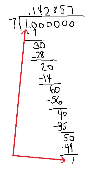
Let’s now return to where this series began… the decimal representation of $\displaystyle \frac{1}{7}$ using long division. As shown below, the repeating block has length $6$ , which can be found in a few minutes with enough patience. By the end of this post, we’ll consider a modification of ordinary long division that facilitates the computation of really long repeating blocks.

Because we arrived at a repeated remainder, we know that we have found the repeating block. So we can conclude that $\displaystyle \frac{1}{7} = 0.\overline{142857}$ .

Students are taught long division in elementary school and are so familiar with the procedure that not much thought is given to the logic behind the procedure. The underlying theorem behind long division is typically called the division algorithm. From Wikipedia:

Given two integers $a$ and $b$ , with $b \ne 0$ , there exist unique integers $q$ and $r$ such that $a = bq+r$ and $0 \le r < |b|$, where $|b|$ denotes the absolute value of $b$ .

The number $q$ is typically called the quotient, while the number $r$ is called the remainder.

Repeated application of this theorem is the basis for long division. For the example above:

Step 1.

$10 = 1 \times 7 + 3$ . Dividing by $10$ , $1 = 0.1 \times 7 + 0.3$

Step 2.

$30 = 4 \times 7 + 2$ . Dividing by $100$ , $0.3 = 0.04 \times 7 + 0.02$

Returning to the end of Step 1, we see that

$1 = 0.1 \times 7 + 0.3 = 0.1 \times 7 + 0.04 \times 7 + 0.02 = 0.14 \times 7 + 0.02$

Step 3.

$20 = 2 \times 7 + 6$ . Dividing by $1000$ , $0.02 = 0.002 \times 7 + 0.006$

Returning to the end of Step 2, we see that

$1 = 0.14 \times 7 + 0.02 = 0.14 \times 7 + 0.0002 \times 7 + 0.006 = 0.142 \times 7 + 0.006$

And so on.

By adding an extra zero and using the division algorithm, the digits in the decimal representation are found one at a time. That said, it is possible (with a calculator) to find multiple digits in a single step by adding extra zeroes. For example:

Alternate Step 1.

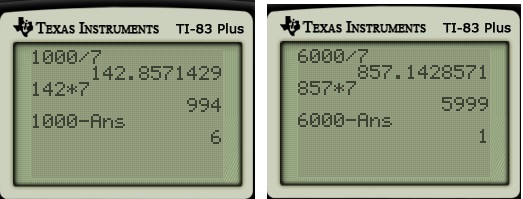
$1000 = 142 \times 7 + 6$ . Dividing by $1000$ , $1 = 0.142 \times 7 + 0.006$

Alternate Step 2.

$6000 = 587 \times 7 + 1$ . Dividing by $100000$ , $0.006 = 0.000587 \times 7 + 0.000001$

Returning to the end of Alternate Step 1, we see that

$1 = 0.142 \times 7 + 0.006= 0.142 \times 7 + 0.000587\times 7 + 0.000001 = 0.142857 \times 7 + 0.000001$

So, with these two alternate steps, we arrive at a remainder of $1$ and have found the length of the repeating block.

The big catch is that, if $a = 1000$ or $a = 6000$ and $b = 7$ , the appropriate values of $q$ and $r$ have to be found. This can be facilitated with a calculator. The integer part of $1000/7$ and $6000/7$ are the two quotients needed above, and subtraction is used to find the remainders (which must be less than $7$ , of course).

At first blush, it seems silly to use a calculator to find these values of $q$ and $r$ when a calculator could have been used to just find the decimal representation of $1/7$ in the first place. However, the advantage of this method becomes clear when we consider fractions who repeating blocks are longer than 10 digits.

Let’s now return to the question posed at the top of this post: finding the decimal representation of $\displaystyle \frac{8}{17}$ . As noted in Part 6 of this series, the length of the repeating block must be a factor of $\phi(17)$ , where $\phi$ is the Euler toitent function, or the number of integers less than $17$ that are relatively prime with $17$ . Since $17$ is prime, we clearly see that $\phi(17) = 16$ . So we can conclude that the length of the repeating block is a factor of $16$ , or either $1$ , $2$ , $4$ , $8$ , or $16$ .

Here’s the result of the calculator again:

We clearly see from the calculator that the repeating block doesn’t have a length less than or equal to $8$ . By process of elimination, the repeating block must have a length of $16$ digits.

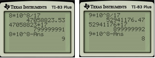
Now we perform the division algorithm to obtain these digits, as before. This can be done in two steps by multiplying by $10^8 = 100,000,000$ .

So, by the same logic used above, we can conclude that

$\displaystyle \frac{8}{17} = 0.\overline{4705882352941176}$

In other words, through clever use of the calculator, the full decimal representation can be quickly found even if the calculator itself returns only ten digits at a time… and had rounded the final $2941176$ of the repeating block up to $3$ .

Calculator errors: When close isn’t close enough (Part 2)

In the previous post, I gave a simple classroom demonstration to illustrate that some calculators only approximate an infinite decimal expansion with a terminating decimal expansion, and hence truncation errors can propagate. This example addresses the common student question, “What’s the big deal if I round off to a few decimal places?”

(For what it’s worth, I’m aware that some current high-end calculators are miniature computer algebra systems and can formally handle an answer of $\displaystyle \frac{1}{3}$ instead of its decimal expansion.)

Students may complain that the above exercise is artificial and unlikely to occur in real life. I would suggest following up with a real-world, non-artificial, and tragic example of an accident that happened in large part due to truncation error. This incident occurred during the first Gulf War in 1991 (perhaps ancient history to today’s students). I’m going to quote directly from the website http://www.ima.umn.edu/~arnold/disasters/patriot.html, published by Dr. Douglas Arnold at the University of Minnesota. Perhaps students don’t need to master the details of this explanation (a binary expansion as opposed to a decimal expansion might be a little abstract), but I think that this example illustrates truncation error vividly.

On February 25, 1991, during the Gulf War, an American Patriot Missile battery in Dharan, Saudi Arabia, failed to track and intercept an incoming Iraqi Scud missile. The Scud struck an American Army barracks, killing 28 soldiers and injuring around 100 other people. A report of the General Accounting office, GAO/IMTEC-92-26, entitled Patriot Missile Defense: Software Problem Led to System Failure at Dhahran, Saudi Arabia reported on the cause of the failure.

It turns out that the cause was an inaccurate calculation of the time since boot due to computer arithmetic errors. Specifically, the time in tenths of second as measured by the system’s internal clock was multiplied by $1/10$ to produce the time in seconds. This calculation was performed using a 24 bit fixed point register. In particular, the value $1/10$ , which has a non-terminating binary expansion, was chopped at 24 bits after the radix point. The small chopping error, when multiplied by the large number giving the time in tenths of a second, led to a significant error.

Indeed, the Patriot battery had been up around 100 hours, and an easy calculation shows that the resulting time error due to the magnified chopping error was about $0.34$ seconds.

The number $1/10$ equals

$\displaystyle \frac{1}{2^4} + \frac{1}{2^5} +\frac{1}{2^8} + \frac{1}{2^9} + \frac{1}{2^{12}} + \frac{1}{2^{13}} + \dots$

In other words, the binary expansion of $1/10$ is

$0.0001100110011001100110011001100....$

Now the 24 bit register in the Patriot stored instead

$0.00011001100110011001100$

introducing an error of

$0.0000000000000000000000011001100...$ binary,

or about $0.000000095$ decimal. Multiplying by the number of tenths of a second in $100$ hours gives

$0.000000095 \times 100 \times 60 \times 60 \times 10=0.34$ .

A Scud travels at about $1,676$ meters per second, and so travels more than half a kilometer in this time. This was far enough that the incoming Scud was outside the “range gate” that the Patriot tracked.

Ironically, the fact that the bad time calculation had been improved in some parts of the code, but not all, contributed to the problem, since it meant that the inaccuracies did not cancel.

The following paragraph is excerpted from the GAO report.

The range gate’s prediction of where the Scud will next appear is a function of the Scud’s known velocity and the time of the last radar detection. Velocity is a real number that can be expressed as a whole number and a decimal (e.g., 3750.2563…miles per hour). Time is kept continuously by the system’s internal clock in tenths of seconds but is expressed as an integer or whole number (e.g., 32, 33, 34…). The longer the system has been running, the larger the number representing time. To predict where the Scud will next appear, both time and velocity must be expressed as real numbers. Because of the way the Patriot computer performs its calculations and the fact that its registers are only 24 bits long, the conversion of time from an integer to a real number cannot be any more precise than 24 bits. This conversion results in a loss of precision causing a less accurate time calculation. The effect of this inaccuracy on the range gate’s calculation is directly proportional to the target’s velocity and the length of the the system has been running. Consequently, performing the conversion after the Patriot has been running continuously for extended periods causes the range gate to shift away from the center of the target, making it less likely that the target, in this case a Scud, will be successfully intercepted.

A quick note of clarification. To verify the binary expansion of $1/10$ , we use the formula for an infinite geometric series.

$S = \displaystyle \left(\frac{1}{2^4} + \frac{1}{2^5}\right) +\left(\frac{1}{2^8} + \frac{1}{2^9}\right) + \left(\frac{1}{2^{12}} + \frac{1}{2^{13}}\right) + \dots$

$S = \displaystyle \frac{3}{2^5} + \frac{3}{2^9} + \frac{3}{2^{13}} + \dots$

$S = \displaystyle \frac{\displaystyle \frac{3}{2^5}}{\quad \displaystyle 1 - \frac{1}{2^4} \quad}$

$S = \displaystyle \frac{\displaystyle \frac{3}{32}}{\quad \displaystyle \frac{15}{16} \quad}$

$S = \displaystyle \frac{3}{32} \times \frac{16}{15}$

$S = \displaystyle \frac{1}{10}$

OK, that verifies the answer. Still, a curious student may wonder how one earth one could directly convert $1/10$ into binary without knowing the above series ahead of time. I will address this question in a future post.

Calculator errors: When close isn’t close enough (Part 1)

Far too often, students settle for a numerical approximation of a solution that can be found exactly. To give an extreme example, I have met quite intelligent college students who were convinced that $\displaystyle \frac{1}{3}$ was literally equal to $0.3$ .

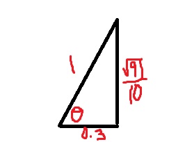
That’s an extreme example of something that nearly all students do — round off a complicated answer to a fixed number of decimal places. In trigonometry, many students will compute $\sin \left( \cos^{-1} 0.3 \right)$ by plugging into a calculator and reporting the first three to six decimal places, like $0.95394$ . This is especially disappointing when there are accessible techniques for getting the exact answer (in this case, $\displaystyle \frac{\sqrt{91}}{10}$ ) without using a calculator at all.

Unfortunately, even maintaining eight, nine, or ten decimal places of accuracy may not be good enough, as errors tend to propagate as a calculation continues. I’m sure every math teacher has an example where the correct answer was exactly $\displaystyle\frac{3}{2}$ but students returned an answer of $1.4927$ or $1.5031$ because of roundoff errors.

Students may ask, “What’s the big deal if I round off to five decimal places?” Here’s a simple example — which can be quickly demonstrated in a classroom — of how such truncation errors can propagate. I’m going to generate a recursive sequence. I will start with $\displaystyle \frac{1}{3}$ . Then I will alternate multiplying by $1000$ and then subtracting $333$ . More mathematically,

$a_1 = \displaystyle \frac{1}{3}$

$a_{2n} = 1000 a_{2n-1}$

$a_{2n+1} = a_{2n} - 333$ if $n > 0$

Here’s what happens exactly:

$1000 \times \displaystyle \frac{1}{3} = \displaystyle \frac{1000}{3} = \displaystyle 333\frac{1}{3} = 333.\overline{3}$

$\displaystyle 333\frac{1}{3} - 333 = \displaystyle \frac{1}{3} = 0.\overline{3}$

So, repeating these two steps, the sequence alternates between $\displaystyle \frac{1}{3}$ and $\displaystyle 333\frac{1}{3}$ .

But looks what happens if I calculate the first twelve terms of this sequence on a calculator.

Notice that by the time I reach $a_{11}$ , the terms of the sequence are negative, which is clearly incorrect.

So what happened?

This is a natural by-product of the finite storage of a calculator. The calculator doesn’t store infinitely many digits of $\displaystyle \frac{1}{3}$ in memory because a calculator doesn’t possess an infinite amount of memory. Instead, what gets stored is something like the terminating decimal $0.33333333333333$ , with about fourteen $3$ s. (Of course, only the first ten digits are actually displayed.)

So multiplying by $1000$ and then subtracting $333$ produces a new and different terminating decimal with three less $3$ s. Do this enough times, and you end up with negative numbers.

Square roots with a calculator (Part 11)

This is the last in a series of posts about square roots and other roots, hopefully providing a deeper look at an apparently simple concept. However, in this post, we discuss how calculators are programmed to compute square roots quickly.

Today’s movie clip, therefore, is set in modern times:

So how do calculators find square roots anyway? First, we recognize that $\sqrt{a}$ is a root of the polynomial $f(x) = x^2 - a$ . Therefore, Newton’s method (or the Newton-Raphson method) can be used to find the root of this function. Newton’s method dictates that we begin with an initial guess $x_1$ and then iteratively find the next guesses using the recursively defined sequence

$x_{n+1} = x_n - \displaystyle \frac{f(x_n)}{f'(x_n)}$

For the case at hand, since $f'(x) = 2x$ , we may write

$x_{n+1} = x_n - \displaystyle \frac{x_n^2 -a}{2 x_n}$ ,

which reduces to

$x_{n+1} = \displaystyle \frac{2x_n^2 - (x_n^2 -a)}{2 x_n} = \frac{x_n^2 + a}{2x_n} = \frac{1}{2} \left( x_n + \frac{a}{x_n} \right)$

This algorithm can be programmed using C++, Python, etc.. For pedagogical purposes, however, I’ve found that a spreadsheet like Microsoft Excel is a good way to sell this to students. In the spreadsheet below, I use Excel to find $\sqrt{2000}$ . In cell A1, I entered $1000$ as a first guess for $\sqrt{2000}$ . Notice that this is a really lousy first guess! Then, in cell A2, I typed the formula

=1/2*(A1+2000/A1)

So Excel computes

$x_2 = \frac{1}{2} \left( x_1 + \displaystyle \frac{2000}{x_1} \right) = \frac{1}{2} \left( 1000 + \displaystyle \frac{2000}{1000} \right) = 501$ .

Then I filled down that formula into cells A3 through A16.

Notice that this algorithm quickly converges to $\sqrt{2000}$ , even though the initial guess was terrible. After 7 steps, the answer is only correct to 2 significant digits ( $45$ ). After 8 steps, the answer is correct to 4 significant digits ( $44.72$ ). On the 9th step, the answer is correct to 9 significant digits ( $44.7213595$ ).

Indeed, there’s a theorem that essentially states that, when this algorithm converges, the number of correct digits basically doubles with each successive step. That’s a lot better than the methods shown at the start of this series of posts which only produced one extra digit with each step.

This algorithm works for finding $k$ th roots as well as square roots. Since $\sqrt[k]{a}$ is a root of $f(x) = x^k - a$ , Newton’s method reduces to

$x_{n+1} = x_n - \displaystyle \frac{x_n^k - a}{k x_n^{k-1}} = \displaystyle \frac{(k-1) x_n^k + a}{k x_n^{k-1}} = \displaystyle \frac{k-1}{k} x_k + \frac{1}{k} \cdot \frac{a}{x_n}$ ,

which reduces to the above sequence if $k =2$ .

See also this Wikipedia page for further historical information as well as discussion about how the above recursive sequence can be obtained without calculus.

Engaging students: Box and whisker plots

In my capstone class for future secondary math teachers, I ask my students to come up with ideas for engaging their students with different topics in the secondary mathematics curriculum. In other words, the point of the assignment was not to devise a full-blown lesson plan on this topic. Instead, I asked my students to think about three different ways of getting their students interested in the topic in the first place.

I plan to share some of the best of these ideas on this blog (after asking my students’ permission, of course).

This submission comes from my former student Jesse Faltys. Her topic: how to engage students when teaching box and whisker plots.

A. Applications – How could you as a teacher create an activity or project that involves your topic?

Students can take a roster of a professional basketball team and create a box and whiskers plot by using the players’ stats of height and weight. As the teacher, you can provide these numbers to them. The weight should be left in pounds, but change the height measurement to inches. The students could be placed in groups of 3 or 4 and given different team rosters. First, have the student calculate the minimum, maximum, lower quartile, upper quartile, and median for their roster for both the weight and height. Then, have the students place the plots on large sheets of paper and present to the class. As the students compare their plots, they can begin to see what effects the range of data has on the construction of each box and whisker plot. Depending on the knowledge of the students you might want them to all working on the same team. As the teacher, you can remove one player’s stats from each group effectively changing the box and whiskers plots and having the students analyzing the data’s effect on the plot constructed from the same roster.

I actually used this in a lesson during my Step II class in a middle school classroom. I used information from the Illuminations website at http://illuminations.nctm.org/LessonDetail.aspx?ID=L737.

B. Curriculum – How can this topic be used in your students’ future courses in mathematics or science?

Any science course with a lab will require you to complete a formal lab write-up. The data collected from your experiment will need to be represented in an organized manner. The features of a box-and-whiskers plot will allow you to gather all your information and make observations off the data that your group and the class as a whole collected. This information can be combined into one plot or the individual lab groups can be compared for any inconsistencies. A box-and-whisker plot can be useful for handling many data values. It shows only certain statistics rather than all the data. Five-number summary is another name for the visual representations of the box-and-whisker plot. The five-number summary consists of the median, the quartiles, and the smallest and greatest values in the distribution. Immediate visuals of a box-and-whisker plot are the center, the spread, and the overall range of distribution. This documentation will allow the student to make a formal analysis while putting together their formal lab write-up.

E. Technology – How can technology be used to effectively engage students with this topic?

1. Khan Academy provides a video titled “Reading Box-and-Whisker Plots” which shows an example of a collection of data on the age of trees. The instructor on the video goes through the representations of the different parts of the structure of the box and whiskers plot. For our listening learners, this reiterates to the student what the plot is summarizing. http://www.khanacademy.org/math/probability/descriptive-statistics/Box-and-whisker%20plots/v/reading-box-and-whisker-plots

2. Math Warehouse allows you to enter the data you are using and it will calculate the plot for you. After having the students work on their own plots, you can have them check their work for themselves. This will allow for immediate confirmation if the student is creating the graph correctly with the data provided. Also, this is allowing the visual learners to see what happens to the length of the box or whiskers when changes are made to the minimum, maximum or median. http://www.mathwarehouse.com/charts/box-and-whisker-plot-maker.php#boxwhiskergraph

3. The Brainingcamp is another website that allows for interaction between the different parts of the plot and the student. This website allows for the students to see a group of data and the matching box-and-whiskers plot. The student can then explore by manually changing different values and instantly seeing a change in the graph. This involvement can stimulate questions to direct the student to complete understanding of the subject. As a hands on learner, it allows the students to manipulate the plot immediately in different “what if” situations. http://www.brainingcamp.com/resources/math/box-plots/interactive.php

Reminding students about Taylor series (Part 6)

Sadly, at least at my university, Taylor series is the topic that is least retained by students years after taking Calculus II. They can remember the rules for integration and differentiation, but their command of Taylor series seems to slip through the cracks. In my opinion, the reason for this lack of retention is completely understandable from a student’s perspective: Taylor series is usually the last topic covered in a semester, and so students learn them quickly for the final and quickly forget about them as soon as the final is over.

Of course, when I need to use Taylor series in an advanced course but my students have completely forgotten this prerequisite knowledge, I have to get them up to speed as soon as possible. Here’s the sequence that I use to accomplish this task. Covering this sequence usually takes me about 30 minutes of class time.

I should emphasize that I present this sequence in an inquiry-based format: I ask leading questions of my students so that the answers of my students are driving the lecture. In other words, I don’t ask my students to simply take dictation. It’s a little hard to describe a question-and-answer format in a blog, but I’ll attempt to do this below.

In the previous posts, I described how I lead students to the definition of the Maclaurin series

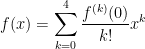
$f(x) = \displaystyle \sum_{k=0}^{\infty} \frac{f^{(k)}(0)}{k!} x^k$ ,

which converges to $f(x)$ within some radius of convergence for all functions that commonly appear in the secondary mathematics curriculum.

Step 7. Let’s now turn to trigonometric functions, starting with $f(x) = \sin x$ .

What’s $f(0)$ ? Plugging in, we find $f(0) = \sin 0 = 0$ .

As before, we continue until we find a pattern. Next, $f'(x) = \cos x$ , so that $f'(0) = 1$ .

Next, $f''(x) = -\sin x$ , so that $f''(0) = 0$ .

Next, $f'''(x) = -\cos x$ , so that $f''(0) = -1$ .

No pattern yet. Let’s keep going.

Next, $f^{(4)}(x) = \sin x$ , so that $f^{(4)}(0) = 0$ .

Next, $f^{(5)}(x) = \cos x$ , so that $f^{(5)}(0) = 1$ .

Next, $f^{(6)}(x) = -\sin x$ , so that $f^{(6)}(0) = 0$ .

Next, $f^{(7)}(x) = -\cos x$ , so that $f^{(7)}(0) = -1$ .

OK, it looks like we have a pattern… albeit more awkward than the patterns for $e^x$ and $\displaystyle \frac{1}{1-x}$ . Plugging into the series, we find that

$\displaystyle \sin x= x - \frac{x^3}{3!} + \frac{x^5}{5!} - \frac{x^7}{7!} \dots$

If we stare at the pattern of terms long enough, we can write this more succinctly as

$\sin x = \displaystyle \sum_{n=0}^\infty (-1)^n \frac{x^{2n+1}}{(2n+1)!}$

The $(-1)^n$ term accounts for the alternating signs (starting on positive with $n=0$ ), while the $2n+1$ is needed to ensure that each exponent and factorial is odd.

Let’s see… $\sin x$ has a Taylor expansion that only has odd exponents. In what other sense are the words “sine” and “odd” associated?

In Precalculus, a function $f(x)$ is called odd if $f(-x) = -f(x)$ for all numbers $x$ . For example, $f(x) = x^9$ is odd since $f(-x) = (-x)^9 = -x^9$ since 9 is a (you guessed it) an odd number. Also, $\sin(-x) = -\sin x$ , and so $\sin x$ is also an odd function. So we shouldn’t be that surprised to see only odd exponents in the Taylor expansion of $\sin x$ .

A pedagogical note: In my opinion, it’s better (for review purposes) to avoid the $\displaystyle \sum$ notation and simply use the “dot, dot, dot” expression instead. The point of this exercise is to review a topic that’s been long forgotten so that these Taylor series can be used for other purposes. My experience is that the $\displaystyle \sum$ adds a layer of abstraction that students don’t need to overcome for the time being.

Step 8. Let’s now turn try $f(x) = \cos x$ .

What’s $f(0)$ ? Plugging in, we find $f(0) = \cos 1 = 0$ .

Next, $f'(x) = -\sin x$ , so that $f'(0) = 0$ .

Next, $f''(x) = -\cos x$ , so that $f'(0) = -1$ .

It looks like the same pattern of numbers as above, except shifted by one derivative. Let’s keep going.

Next, $f'''(x) = \sin x$ , so that $f'''(0) = 0$ .

Next, $f^{(4)}(x) = \cos x$ , so that $f^{(4)}(0) = 1$ .

Next, $f^{(5)}(x) = -\sin x$ , so that $f^{(5)}(0) = 0$ .

Next, $f^{(6)}(x) = -\cos x$ , so that $f^{(6)}(0) = -1$ .

OK, it looks like we have a pattern somewhat similar to that of $\sin x$, except only involving the even terms. I guess that shouldn’t be surprising since, from precalculus we know that $\cos x$ is an even function since $\cos(-x) = \cos x$ for all $x$ .

Plugging into the series, we find that

$\displaystyle \cos x= 1 - \frac{x^2}{2!} + \frac{x^4}{4!} - \frac{x^6}{6!} \dots$

If we stare at the pattern of terms long enough, we can write this more succinctly as

$\cos x = \displaystyle \sum_{n=0}^\infty (-1)^n \frac{x^{2n}}{(2n)!}$

As we saw with $e^x$ , the above series converge quickest for values of $x$ near $0$ . In the case of $\sin x$ and $\cos x$ , this may be facilitated through the use of trigonometric identities, thus accelerating convergence.

For example, the series for $\cos 1000^o$ will converge quite slowly (after converting $1000^o$ into radians). However, we know that

$\cos 1000^o= \cos(1000^o - 720^o) =\cos 280^o$

using the periodicity of $\cos x$ . Next, since $\latex 280^o$ is in the fourth quadrant, we can use the reference angle to find an equivalent angle in the first quadrant:

$\cos 1000^o = \cos 280^o = \cos(360^o - 80^o) = \cos 80^o$

Finally, using the cofunction identity $\cos x = \sin(90^o - x)$ , we find

$\cos 1000^o = \cos 80^o = sin(90^o - 80^o) = \sin 10^o$ .

In this way, the sine or cosine of any angle can be reduced to the sine or cosine of some angle between $0^o$ and $45^o = \pi/4$ radians. Since $\pi/4 < 1$ , the above power series will converge reasonably rapidly.

Step 10. For the final part of this review, let’s take a second look at the Taylor series

$e^x = \displaystyle 1 + x + \frac{x^2}{2} + \frac{x^3}{3} + \frac{x^4}{4} + \frac{x^5}{5} + \frac{x^6}{6} + \frac{x^7}{7} + \dots$

Just to be silly — for no apparent reason whatsoever, let’s replace $x$ by $ix$ and see what happens:

$e^{ix} = \displaystyle 1 - \frac{x^2}{2!} + \frac{x^4}{4!} - \frac{x^6}{6!} \dots + i \left[\displaystyle x - \frac{x^3}{3!} + \frac{x^5}{5!} - \frac{x^7}{7!} \dots \right]$

after separating the terms that do and don’t have an $i$ .

Hmmmm… looks familiar….

So it makes sense to define

$e^{ix} = \cos x + i \sin x$ ,

which is called Euler’s formula, thus proving an unexpected connected between $e^x$ and the trigonometric functions.

Reminding students about Taylor series (Part 4)

I’m in the middle of a series of posts describing how I remind students about Taylor series. In the previous posts, I described how I lead students to the definition of the Maclaurin series

$f(x) = \displaystyle \sum_{k=0}^{\infty} \frac{f^{(k)}(0)}{k!} x^k$ ,

which converges to $f(x)$ within some radius of convergence for all functions that commonly appear in the secondary mathematics curriculum.

Step 4. Let’s now get some practice with Maclaurin series. Let’s start with $f(x) = e^x$ .

What’s $f(0)$ ? That’s easy: $f(0) = e^0 = 1$ .

Next, to find $f'(0)$ , we first find $f'(x)$ . What is it? Well, that’s also easy: $f'(x) = \frac{d}{dx} (e^x) = e^x$ . So $f'(0)$ is also equal to $1$ .

How about $f''(0)$ ? Yep, it’s also $1$ . In fact, it’s clear that $f^{(n)}(0) = 1$ for all $n$ , though we’ll skip the formal proof by induction.

Plugging into the above formula, we find that

$e^x = \displaystyle \sum_{k=0}^{\infty} \frac{1}{k!} x^k = \sum_{k=0}^{\infty} \frac{x^k}{k!} = 1 + x + \frac{x^2}{2} + \frac{x^3}{3} + \dots$

It turns out that the radius of convergence for this power series is $\infty$ . In other words, the series on the right converges for all values of $x$ . So we’ll skip this for review purposes, this can be formally checked by using the Ratio Test.

At this point, students generally feel confident about the mechanics of finding a Taylor series expansion, and that’s a good thing. However, in my experience, their command of Taylor series is still somewhat artificial. They can go through the motions of taking derivatives and finding the Taylor series, but this complicated symbol in $\displaystyle \sum$ notation still doesn’t have much meaning.

So I shift gears somewhat to discuss the rate of convergence. My hope is to deepen students’ knowledge by getting them to believe that $f(x)$ really can be approximated to high precision with only a few terms. Perhaps not surprisingly, it converges quicker for small values of $x$ than for big values of $x$ .

Pedagogically, I like to use a spreadsheet like Microsoft Excel to demonstrate the rate of convergence. A calculator could be used, but students can see quickly with Excel how quickly (or slowly) the terms get smaller. I usually construct the spreadsheet in class on the fly (the fill down feature is really helpful for doing this quickly), with the end product looking something like this:

In this way, students can immediately see that the Taylor series is accurate to four significant digits by going up to the $x^4$ term and that about ten or eleven terms are needed to get a figure that is as accurate as the precision of the computer will allow. In other words, for all practical purposes, an infinite number of terms are not necessary.

In short, this is how a calculator computes $e^x$ : adding up the first few terms of a Taylor series. Back in high school, when students hit the $e^x$ button on their calculators, they’ve trusted the result but the mechanics of how the calculator gets the result was shrouded in mystery. No longer.

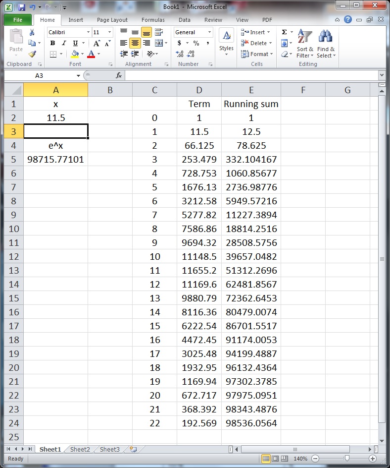
Then I shift gears by trying a larger value of $x$ :

I ask my students the obvious question: What went wrong? They’re usually able to volunteer a few ideas:

The convergence is slower for larger values of $x$ .
The series will converge, but more terms are needed (and I’ll later use the fill down feature to get enough terms so that it does converge as accurate as double precision will allow).
The individual terms get bigger until $k=11$ and then start getting smaller. I’ll ask my students why this happens, and I’ll eventually get an explanation like

$\displaystyle \frac{(11.5)^6}{6!} < \frac{(11.5)^6}{6!} \times \frac{11.5}{7} = \frac{(11.5)^7}{7!}$

but

$\displaystyle \frac{(11.5)^{11}}{11!} < \frac{(11.5)^{11}}{11!} \times \frac{11.5}{12} = \frac{(11.5)^{12}}{12!}$

At this point, I’ll mention that calculators use some tricks to speed up convergence. For example, the calculator can simply store a few values of $e^x$ in memory, like $e^{16}$ , $e^{8}$ , $e^{4}$ , $e^{2}$ , and $e^{1} = e$ . I then ask my class how these could be used to find $e^{11.5}$ . After some thought, they will volunteer that

$e^{11.5} = e^8 \cdot e^2 \cdot e \cdot e^{0.5}$ .

The first three values don’t need to be computed — they’ve already been stored in memory — while the last value can be computed via Taylor series. Also, since $0.5 < 1$ , the series for $e^{0.5}$ will converge pretty quickly. (Some students may volunteer that the above product is logically equivalent to turning $11$ into binary.)

At this point — after doing these explicit numerical examples — I’ll show graphs of $e^x$ and graphs of the Taylor polynomials of $e^x$ , observing that the polynomials get closer and closer to the graph of $e^x$ as more terms are added. (For example, see the graphs on the Wikipedia page for Taylor series, though I prefer to use Mathematica for in-class purposes.) In my opinion, the convergence of the graphs only becomes meaningful to students only after doing some numerical examples, as done above.

At this point, I hope my students are familiar with the definition of Taylor (Maclaurin) series, can apply the definition to $e^x$ , and have some intuition meaning that the nasty Taylor series expression practically means add a bunch of terms together until you’re satisfied with the convergence.

In the next post, we’ll consider another Taylor series which ought to be (but usually isn’t) really familiar to students: an infinite geometric series.

P.S. Here’s the Excel spreadsheet that I used to make the above figures: Taylor.

Reminding students about Taylor series (Part 3)

In the previous post, I described how I lead students to the equations

$f(x) = \displaystyle \sum_{k=0}^n \frac{f^{(k)}(0)}{k!} x^k$ .

and

$f(x) = \displaystyle \sum_{k=0}^n \frac{f^{(k)}(a)}{k!} (x-a)^k$ ,

where $f(x)$ is a polynomial and $a$ can be any number.

Step 3. What happens if the original function $f(x)$ is not a polynomial? For one thing, the right-hand side can no longer be a finite sum. As long as the sum on the right-hand side stops at some degree $n$ , the right-hand side is a polynomial, but the left-hand side is assumed to not be a polynomial.

To resolve this, we can cross our fingers and hope that

$f(x) = \displaystyle \sum_{k=0}^{\infty} \frac{f^{(k)}(0)}{k!} x^k$ ,

$f(x) = \displaystyle \sum_{k=0}^{\infty}\frac{f^{(k)}(a)}{k!} (x-a)^k$ .

In other words, let’s make the right-hand side an infinite series, and hope for the best. This is the definition of the Taylor series expansions of $f$ .

Note: At this point in the review, I can usually see the light go on in my students’ eyes. Usually, they can now recall their work with Taylor series in the past… and they wonder why they weren’t taught this topic inductively (like I’ve tried to do in the above exposition) instead of deductively (like the presentation in most textbooks).

While we’d like to think that the Taylor series expansions always work, there are at least two things that can go wrong.

First, the sum on the left is an infinite series, and there’s no guarantee that the series will converge in the first place. There are plenty of example of series that diverge, like $\displaystyle \sum_{k=0}^\infty \frac{1}{k+1}$ .
Second, even if the series converges, there’s no guarantee that the series will converge to the “right” answer $f(x)$ . The canonical example of this behavior is $f(x) = e^{-1/x^2}$ , which is so “flat” near $x=0$ that every single derivative of $f$ is equal to $0$ at $x =0$ .

For the first complication, there are multiple tests devised in Calculus II, especially the Ratio Test, to determine the values of $x$ for which the series converges. This establishes a radius of convergence for the series.

The second complication is far more difficult to address rigorously. The good news is that, for all commonly occurring functions in the secondary mathematics curriculum, the Taylor series of a function properly converges (when it does converge). So we will happily ignore this complication for the remainder of the presentation.

Indeed, it’s remarkable that the series should converge to $f(x)$ at all. Think about the meaning of the terms on the right-hand side:

$f(a)$ is the $y-$ coordinate at $x=a$ .
$f'(a)$ is the slope of the curve at $x=a$ .
$f''(a)$ is a measure of the concavity of the curve at — you guessed it — $x=a$ .
$f'''(a)$ is an even more subtle description of the curve… once again, at $x=a$ .

In other words, if the Taylor series converges to $f(x)$ , then every twist and turn of the function, even at points far away from $x=a$ , is encoded somehow in the shape of the curve at the one point $x=a$ . So analytic functions (which has a Taylor series which converges to the original functions) are indeed quite remarkable.

Reminding students about Taylor series (Part 2)

In this series of posts, I will describe the sequence of examples that I use to remind students about Taylor series. (One time, just for fun, I presented this topic at the end of a semester of Calculus I, and it seemed to go well even for that audience who had not seen Taylor series previously.)

I should emphasize that I present this sequence inductively and in an inquiry-based format: I ask leading questions of my students so that the answers of my students are driving the lecture. In other words, I don’t ask my students to simply take dictation. It’s a little hard to describe a question-and-answer format in a blog, but I’ll attempt to do this below.

Step 1. Find the unique quartic (fourth-degree) polynomial so that $f(0) = 6$ , $f'(0) = -3$ , $f''(0) = 6$ , $f'''(0) = 2$ , and $f^{(4)}(0) = 10$ .

I’ve placed a thought bubble if you’d like to think about it before scrolling down to see the answer. Here’s a hint to get started: let $f(x) = ax^4 + bx^3 + cx^2 + dx + e$ , and start differentiating. Remember that $a$ , $b$ , $c$ , $d$ , and $e$ are constants.

We begin with the information that $f(0) = 6$ . How else can we find $f(0)$? Since $f(x) = ax^4 + bx^3 + cx^2 + dx + e$ , we see that $f(0) = e$ . Therefore, it must be that $e = 6$ .

How about $f'(0)$ ? We see that $f'(x) = 4ax^3 + 3bx^2 + 2cx + d$ , and so $f'(0) = d$ . Since $f'(0) = -3$ , we have that $d = -3$ .

Next, $f''(x) = 12ax^2 + 6bx + 2c$ , and so $f''(0) = 2c$ . Since $f''(0) = 6$ ,we have that $2c = 6$ , or $c = 3$ .

Next, $f'''(x) = 24ax + 6b$ , and so $f'''(0) = 6b$ . Since $f'''(0) = 2$ ,we have that $6b = 2$ , or $b = \frac{1}{3}$ .

Finally, $f^{(4)}(x) = 24a$ , and so $f^{(4)}(0) = 24a$ . Since $f^{(4)}(0) = 10$ , we have $24a = 10$ , or $a = \frac{5}{12}$ .

What do we get when we put all of this information together? The polynomial must be

$f(x) = \frac{5}{12} x^4 + \frac{1}{3} x^3 + 3 x^2 - 3x + 6$ .

Step 2. How are these coefficients related to the information given in the problem?

Let’s start with the leading coefficient, $a = \frac{5}{12}$ . How did we get this answer? It came from dividing $10$ by $24$ . Where did the $10$ come from? It was the given value of $f^{(4)}(0)$ , and so

$a = \displaystyle \frac{f^{(4)}(0)}{24}$ .

Next, $b = \frac{1}{3}$ , which arose from dividing $2$ by $6$ . The number $2$ was the given value of $f'''(0)$ , and so

$b =\displaystyle \frac{f'''(0)}{6}$ .

Moving to the next coefficient, $c = 3$ , which arose from dividing $f''(0) = 6$ by $2$ . So

$c = \displaystyle\frac{f''(0)}{2}$ .

Finally, it’s clear that

$d = f'(0)$ and $e = f(0)$ .

This last line doesn’t quite fit the pattern of the first three lines. The first three lines all have fractions, but these last two expressions don’t. How can we fix this? In the hopes of finding a pattern, let’s (unnecessarily) write $d$ and $e$ as fractions by dividing by $1$ :

$d = \displaystyle\frac{f'(0)}{1}$ and $e = \displaystyle \frac{f(0)}{1}$ .

Let’s now rewrite the polynomial $f(x)$ in light of this discussion:

$f(x) = \displaystyle \frac{f'^{(4)}(0)}{24} x^4 + \frac{f'''(0)}{6} x^3 + \frac{f'''(0)}{2} x^2 + \frac{f'(0)}{1}x + \frac{f(0)}{1}$ .

What pattern do we see in the numerators? It’s apparent that the number of derivatives matches the power of $x$ . For example, the $x^3$ term has a coefficient involving the third derivative of $f$ . The last two terms fit this pattern as well, since $x = x^1$ and the last term is multiplied by $x^0 = 1$ .

What pattern do we see in the denominators? $1, 1, 2, 6, 24 \dots$ where have we seen those before? Oh yes, the factorials! We know that $4! = 4 \cdot 3 \cdot 2 \cdot 1 = 24$ , $3! = 3 \cdot 2 \cdot 1 = 6$ , $2! = 2 \cdot 1 = 2$ , $1! = 1$ , and $0!$ is defined to be $1$ . So $f(x)$ can be rewritten as

$f(x) = \displaystyle \frac{f'^{(4)}(0)}{4!} x^4 + \frac{f'''(0)}{3!} x^3 + \frac{f'''(0)}{2!} x^2 + \frac{f'(0)}{1!}x + \frac{f(0)}{0!}$ .

How can this be written more compactly? By using $\displaystyle \sum-$ notation:

$f(x) = \displaystyle \sum_{k=0}^4 \frac{f^{(k)}(0)}{k!} x^k$ .

Why does the sum stop at 4? Because the original polynomial had degree 4. In general, if the polynomial had degree $n$ , it’s reasonable to guess that

$f(x) = \displaystyle \sum_{k=0}^n \frac{f^{(k)}(0)}{k!} x^k$ .

This is called the Maclaurian series, or the Taylor series about $x =0$ . While I won’t prove it here, one can find Taylor series expansions about points other than $0$ :

$f(x) = \displaystyle \sum_{k=0}^n \frac{f^{(k)}(a)}{k!} (x-a)^k$ ,

where $a$ can be any number. Though not proven here, these series are exactly true for polynomials.

In the next post, we’ll discuss what happens if $f(x)$ is not a polynomial.

Reminding students about Taylor series (Part 1)

At my university, Calculus II covers approximately the same topics covered in an AP Calculus BC course: integrals and derivatives with logarithms and exponential functions, various techniques of integration (including integration by parts and trigonometric substitutions), and convergence of infinite series.

In my opinion, the single most important of these topics is Taylor series (or, if you prefer, Maclaurin series), as these approximations to transcendental functions like $e^x$ and $\sin x$ are used over and over again in higher mathematics.

$\bullet$ A good working knowledge of Taylor series is necessary for computing series solutions of ordinary differential equations.

$\bullet$ In physics, elementary approximations like $\sin x \approx x$ are used over and over again. For example, the governing differential equation for the motion of oscillating pendulums is

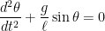
$\displaystyle \frac{d^2 \theta}{dt^2} + \frac{g}{\ell} \sin \theta = 0$ ,

where $g$ is the acceleration due to gravity and $\ell$ is the length of the pendulum. This differential equation cannot be solved exactly, and its solution is very complex.

However, for small angles, we may use the approximation $\sin \theta \approx \theta$ , so that the differential equation becomes

$\displaystyle \frac{d^2 \theta}{dt^2} + \frac{g}{\ell} \theta = 0$ ,

By eliminating the $\sin \theta$ term, we now have a second-order differential equation with constant coefficients, which can be solved in a straightforward manner using standard techniques from differential equations. If $\theta(0) = \theta_0$ and $\theta'(0) = 0$ (i.e., the pendulum is pulled a small angle $\theta_0$ and is then released), the solution is

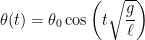
$\theta(t) = \theta_0 \cos\left(t \sqrt{\displaystyle \frac{g}{\ell}} \right)$ .

In other words, the pendulum exhibits sinusoidal behavior. (FYI, for an amazing display of kinetic art, see this demonstration of pendulum waves.)

$\bullet$ The primary way that students interface with Taylor series is through their calculators. When a calculator computes $\cos 1000^o$ , it doesn’t draw a unit circle, trace out an angle of $1000^o$ in standard position, and find the $x-$ coordinate of the terminal point. Instead, the calculator converts $1000^o$ into radians and adds the first few terms of the Taylor series expansion for $\cos x.$

The calculator may use a few tricks to accelerate convergence. For this example, using some trigonometric identities, $\cos 1000^o= \cos 280^o= \cos 80^o= \sin 10^o$ , and (as I’ll discuss) the Maclaurin series for $\sin x$ at $x = 10^o$ converges much faster than the Maclaurin series for $\cos x$ at $x = 1000^o$ .

I’ve argued the importance of Taylor series in higher-level courses in both mathematics and physics. Sadly, at least at my university, Taylor series is probably the topic that is least retained by students years after taking Calculus II. They can remember the rules for integration and differentiation, but their command of Taylor series seems to slip through the cracks.

In my opinion, the reason for this lack of retention is completely understandable from a student’s perspective: Taylor series is usually the last topic covered in a semester, and so students learn them quickly for the final and quickly forget about them as soon as the final is over.

Of course, when I need to use Taylor series in an advanced course but my students have completely forgotten this prerequisite knowledge, I have to get them up to speed as soon as possible. Over the next few posts, I will present the sequence of examples that I use to accomplish this task. Covering this sequence usually takes me about 30-40 minutes of class time, depending on the class.

I should emphasize that, as much as possible, I present this sequence inductively and in an inquiry-based format: I ask leading questions of my students so that the answers of my students are driving the lecture. In other words, I don’t ask my students to simply take dictation. It’s a little hard to describe a question-and-answer format in a blog, but I’ll attempt to do this below.

Beginning with the next post, I’ll describe this sequence.