Arithmetic with big numbers (Part 2)

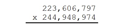
Ready for an elementary arithmetic problem? Here it is:

Nothing to it… just multiply the two numbers. Of course, we’d rather not multiply them by hand, so let’s use a calculator instead:

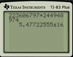
bigmult2

Uh oh… the calculator doesn’t give the complete answer. It does return the first nine significant digits, but it doesn’t return all 16 digits. Indeed, we can’t be sure that the final 5 in the answer is correct because of rounding.

So now what we do (other than buy a more expensive calculator)?

In yesterday’s post, I posed a similar problem involving addition. Adding two big numbers by hand is no big deal. However, multiplying two big numbers, one digit at time, would be tedious!

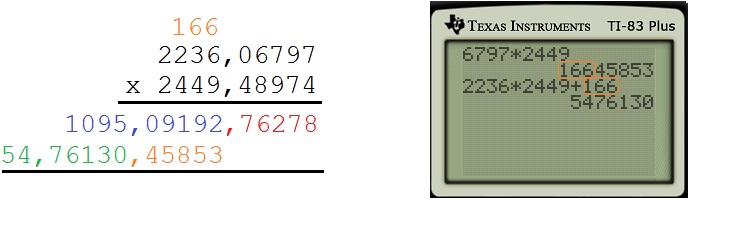
When I pose this question to students, the knee-jerk reaction is to groan when facing the prospect of multiplying these two big numbers by hand. However, it is possible to use modern technology to make ordinary grade-school multiplication move a lot quicker. Perhaps the fastest way to do this is to split the numbers into block of five digits instead of the usual three:

Now we proceed as if each block of five digits was a single digit. We begin with the last block of digits on the second row, which is 48974. First, we multiply 6797 and 48974 using a calculator. Because most modern scientific calculators have a 10-digit display, we can be assured that the complete answer will be shown. (This is why I chose to divide the numbers using block of five digits and not six or more.) The last five digits in the answer are written down; the more significant digits are carried.

Next, we multiply 2236 and 48974 and then add the number that was carried.

bigmult4 We then repeat using 2449, the next (and final) block of digits on the second row. First, we multiply 6797 and 2449 using a calculator. The last five digits in the answer are written down; the more significant digits are carried.

Next, we multiply 2236 and 2449 and then add the number that was carried.

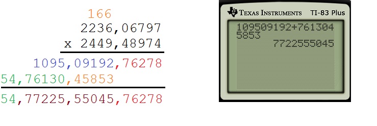
Finally, it remains to add these two partial products to obtain the final product. For this problem, this can be accomplished with only a single addition: the block of digits 76278 simply carry down to the final answer, and so we can start by adding the second and third blocks of digits. As this sum is less than $10^{10}$ , there is no digit to carry, and so the leading 54 also carries down to the final answer.

The above technique is logically equivalent to using base 100,000 as opposed to the customary use of base 10 arithmetic. So while multiplying two numbers in the billions still takes some time, judiciously using a calculator makes this exercise go a lot quicker than the ordinary grade-school method of multiplying one digit at a time.

Arithmetic with big numbers (Part 1)

Ready for an elementary arithmetic problem? Here it is:

Nothing to it… just add the two numbers. Of course, we’d rather not add them by hand, so let’s use a calculator instead:

bigadd5

So now what we do (other than buy a more expensive calculator)?

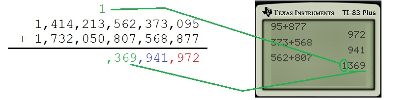
When I pose this question to students, the knee-jerk reaction is to just start adding one digit at a time. Though that’s not the worst possible response, it is possible to use modern technology to make ordinary grade-school addition move a lot quicker. One way to do this is to take three digits at a time while using a calculator:

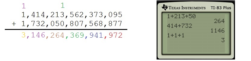
Notice that the 1 in 1369 gets carried over to the next block of three digits in much the same way that a sum greater than 10 has the tens digit carried over to the next digit. Continuing:

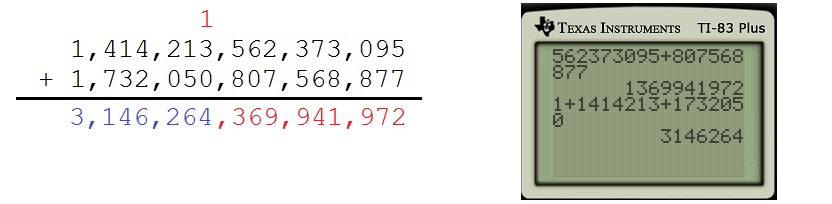
This is logically equivalent to using base 1000 to add these two numbers (as opposed to base 10) and is certainly a lot faster than using only one digit at a time. Of course, it’d go even faster if we use up to nine digits a time (which is equivalent to using base one billion).

Inverse Functions: Logarithms and Complex Numbers (Part 30)

Ordinarily, there are no great difficulties with logarithms as we’ve seen with the inverse trigonometric functions. That’s because the graph of $y = a^x$ satisfies the horizontal line test for any $0 < a < 1$ or $a > 1$ . For example,

$e^x = 5 \Longrightarrow x = \ln 5$ ,

and we don’t have to worry about “other” solutions.

However, this goes out the window if we consider logarithms with complex numbers. Recall that the trigonometric form of a complex number $z = a+bi$ is

$z = r(\cos \theta + i \sin \theta) = r e^{i \theta}$

where $r = |z| = \sqrt{a^2 + b^2}$ and $\tan \theta = b/a$ , with $\theta$ in the appropriate quadrant. This is analogous to converting from rectangular coordinates to polar coordinates.

Over the past few posts, we developed the following theorem for computing $e^z$ in the case that $z$ is a complex number.

Definition. Let $z = r e^{i \theta}$ be a complex number so that $-\pi < \theta \le \theta$ . Then we define

$\log z = \ln r + i \theta$ .

Of course, this looks like what the definition ought to be if one formally applies the Laws of Logarithms to $r e^{i \theta}$ . However, this complex logarithm doesn’t always work the way you’d think it work. For example,

$\log \left(e^{2 \pi i} \right) = \log (\cos 2\pi + i \sin 2\pi) = \log 1 = \ln 1 = 0 \ne 2\pi i$ .

This is analogous to another situation when an inverse function is defined using a restricted domain, like

$\sqrt{ (-3)^2 } = \sqrt{9} = 3 \ne -3$

$\sin^{-1} (\sin \pi) = \sin^{-1} 0 = 0 \ne \pi$ .

The Laws of Logarithms also may not work when nonpositive numbers are used. For example,

$\log \left[ (-1) \cdot (-1) \right] = \log 1 = 0$ ,

but

$\log(-1) + \log(-1) = \log \left( e^{\pi i} \right) + \log \left( e^{\pi i} \right) = \pi i + \pi i = 2\pi i$ .

green line

This material appeared in my previous series concerning calculators and complex numbers: https://meangreenmath.com/2014/07/09/calculators-and-complex-numbers-part-21/

Inverse Functions: Arcsine (Part 9)

I’d like to discuss a common mistake students make in trigonometry… as well as the one-liner that I use to (hopefully) help students not make this mistake in the future.

Question. Find all solutions (rounded to the nearest tenth of a degree) of $\sin x = 0.8$ .

Erroneous Solution. Plugging into a calculator, we find that $x \approx 53.1^o$ .

I offer a thought bubble if you’d like to think about why this answer is wrong.

The student correctly found the unique angle $x$ between $-90^o$ and $90^o$ so that $\sin x = 0.8$ . That’s the definition of the arcsine function. However, there are plenty of other angles whose sine is equal to $0.7$ . This can happen in two ways.

First, if $\sin x > 0$, then the angle $x$ could be in either the first quadrant or the second quadrant (thanks to the mnemonic All Scholars Take Calculus). So $x$ could be (accurate to one decimal place) equal to either $53.1^o$ or else $180^o - 53.1^o = 126.9^o$ . Students can visualize this by drawing a picture, talking through each step of its construction (first black, then red, then brown, then green, then blue).

However, most students really believe that there’s a second angle that works when they see the results of a calculator.

Second, any angle that’s coterminal with either of these two angles also works. This can be drawn into the above picture and, as before, confirmed with a calculator.

So the complete answer (again, approximate to one decimal place) should be $53.1^{\circ} + 360n^o$ and $126.9 + 360n^{\circ}$, where $n$ is an integer. Since integers can be negative, there’s no need to write $\pm$ in the solution.

Therefore, the student who simply answers $53.1^o$ has missed infinitely many solutions. The student has missed every nontrivial angle that’s coterminal with $53.1^o$ and also every angle in the second quadrant that also works.

Here’s my one-liner — which never fails to get an embarrassed laugh — that hopefully helps students remember that merely using the arcsine function is not enough for solving problems such as this one.

You’ve forgotten infinitely many solutions. So how many points should I take off?

Exponential growth and decay (Part 16): Logistic growth model

Today, I discuss the logistic growth model, which describes how an infection (like a disease, a rumor, or advertise) spreads in a population. In yesterday’s post, I described an in-class demonstration that engages students while also making the following formula believable:

$A(t) = \displaystyle \frac{Ly_0}{y_0+ (L-y_0)e^{-rt}}$ .

I’d like to discuss some observations about this somewhat complicated function that will make producing its graph easier. The first two observations are within reach of Precalculus students.

1. Let’s figure out the $y-$ intercept:

$A(0) = \displaystyle \frac{Ly_0}{y_0+ (L-y_0)e^{-r \cdot 0}} = \displaystyle \frac{Ly_0}{y_0+ L-y_0} = y_0$ .

In other words, the number $y_0$ represents the initial number of people who have the infection.

2. Let’s figure out the limiting value as $t$ gets large:

$\displaystyle \lim_{t \to \infty} A(t) = \displaystyle \frac{Ly_0}{y_0+ (L-y_0) \cdot 0} = \displaystyle \frac{Ly_0}{y_0} = L$ .

As expected, all $L$ people will get the infection eventually. (Of course, Precalculus students won’t be familiar with the $\displaystyle \lim$ notation, but they should understand that $e^{-rt}$ decays to zero as $t$ gets large.

3. Let’s now figure out the point of inflection. Ordinarily, points of inflection are found by setting the second derivative equal to zero. Though this can be done for the function $A(t)$ above, it would be a somewhat daunting exercise!

The good news is that the points of inflection can be found quite simply using the governing differential equation, which is

$A' = r A [ L - A] = r L A - r A^2$

Let’s take the derivative of both sides, remembering that $r$ and $L$ are constants:

$A'' = r L A' - 2 r A A'$

$A'' = A' (r L - 2 r A)$

So the second derivative is equal to zero when either $A' = 0$ or else $r L - 2 r A = 0$ . The first case corresponds to the trivial cases $A(t) \equiv 0$ and $A(t) \equiv L$ ; these constants are called the equilibrium solutions. The second case is the more interesting one:

$r L - 2 r A = 0$

$r L = 2 r A$

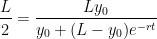
$\displaystyle \frac{L}{2} = A$

This suggests that, as the infection spreads throughout a population, the curve changes concavity at the time that half of the population becomes infected. In other words, the infection spreads fastest throughout the population at the time when half of the population has been infected.

The time at which the point of inflection occurs can be found by setting $A(t) = \displaystyle \frac{L}{2}$ and solving for $t$ :

$\displaystyle \frac{L}{2} = \displaystyle \frac{Ly_0}{y_0+ (L-y_0)e^{-rt}}$ .

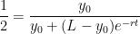
$\displaystyle \frac{1}{2} = \displaystyle \frac{y_0}{y_0+ (L-y_0)e^{-rt}}$ .

$y_0 + (L-y_0) e^{-rt} = 2y_0$

$(L-y_0) e^{-rt} = y_0$

$e^{-rt} = \displaystyle \frac{y_0}{L-y_0}$

$-rt = \displaystyle \ln \left( \frac{y_0}{L-y_0} \right)$

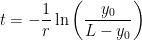
$t = \displaystyle - \frac{1}{r} \ln \left( \frac{y_0}{L-y_0} \right)$

This technique for finding the points of inflection directly from the differential equation is possible whenever the differential equation is autonomous, which loosely means that the independent variable does not appear on the right-hand side.

Exponential growth and decay (Part 15): Logistic growth model

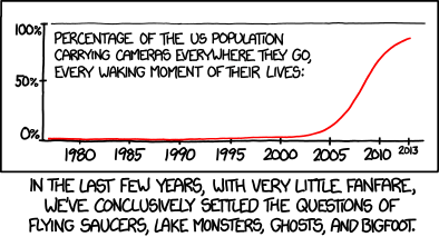
Today, I introduce the logistic growth model, which describes how an infection (like a disease, a rumor, or advertise) spreads in a population. For example:

Sources: http://www.xkcd.com/1220/ and http://www.xkcd.com/1235/

In yesterday’s post, I described an in-class demonstration that engages students while also making the following formula believable:

$A(t) = \displaystyle \frac{L}{1 + (L-1)e^{-rt}}$ .

Where does this formula come from? Suppose that a disease is spreading in a population of size $L$ . It stands to reason that the rate at which the disease spreads is proportional to the number of possible contacts between those who have the disease and those who don’t. If $A(t)$ is the number of people who have the disease, then $L-A(t)$ is the number of people who don’t have the disease. Therefore, the product $A(t) [ L - A(t) ]$ is the number of possible contacts between those who have the disease and those who don’t. This leads to the governing differential equation

$A'(t) = c A(t) [ L - A(t) ]$ ,

where $c$ is the constant of proportionality. This is often rewritten by letting $c = \displaystyle \frac{r}{L}$ , or $r = cL$ :

$A'(t) = \displaystyle \frac{r}{L} A(t) [ L - A(t) ]$

$A'(t) = r A(t) \displaystyle \left[1 - \frac{A(t)}{L} \right]$

The good news is that this differential equation can be solved using separation of variables, just like the governing differential equations for continuous compound interest, paying off credit card debt, radioactive decay, and Newton’s Law of Cooling. The bad news is that it’s a lot harder to calculate the required integrals! After all, the right-hand side, after distributing, has a term containing $A^2$ , which makes this differential equation non-linear.

Solving this differential equation is a bit tedious, and I don’t feel particularly obligated to re-invent the wheel since it can be found several places on the Internet. Suffice it to say that integration by partial fractions and some very tricky algebra is necessary to solve for $A(t)$ and obtain the solution above. Among several different sources (which likely use different letters than the ones I’m using here):

Wikipedia: http://en.wikipedia.org/wiki/Logistic_function#In_ecology:_modeling_population_growth

MathWorld: http://mathworld.wolfram.com/LogisticEquation.html

Exponential growth and decay (Part 14): Logistic growth model

Today, I introduce the logistic growth model, which describes how an infection (like a disease, a rumor, or advertise) spreads in a population. Before I actually present the formula to my students, I usually perform a 8- to 10-minute demonstration to convince students that the formula actually works. This demonstration works well with between 15 and 45 students; I have personally not attempted this demo with a class larger than 45.

I wish I could take credit for the idea behind this demonstration. I’m afraid I can’t remember who told me the idea behind this demo about 15 years ago, but I’m thankful to him or her for this idea, as I’ve used it with great success over the years when teaching Precalculus and even when teaching Differential Equations.

Here’s the demonstration:

1. The class period before the demo, I ask my students to bring their calculators to class.

2. On the day of the demo, I prepare slips of paper with the numbers 1, 2, 3, etc. I hand these to my students as they take their seats before class starts (and, as needed, to students who arrive late).

3. I tell the class that we’re going to model how a rumor gets spread. On the chalkboard, I write down the numbers 0, 1, 2, …, up to $N$ , the number of students in the class that day. Invariably, I get asked, “What’s the rumor?” In response, I’ll playfully point to someone in the front row and say, “The rumor is about him.”

4. I point out that, at time 0, only one person has heard the rumor…. me. I’m person number 0 (confirming the popular belief of my students). So I’ll cross out the 0 on the board and mark on a table that only one person has heard the rumor so far. (Here’s the spreadsheet that I’ve used to keep track of this information while simultaneously making a graph of the data: logisitic).

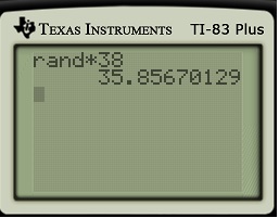
5. I begin to spread the rumor. To spread the rumor, I use my calculator to get a random number between $0$ and $N$ . This can be done by just using the built-in random number generator found on many calculators and then multiplying by $N+1$ . (After all, there are $L= N+1$ people in the room: $N$ students plus one instructor.) The part after the decimal point is not important; the number before the decimal point represents the next person to hear the rumor.

For example, in the figure below, I would tell that person #35 of my class of 37 students was the next to hear the rumor. (If my random number is 0, I’ll privately cheat and get until I get a random number other than 0. I only permit the possibility of cheating on the first step so that the data fits the predicted curve as accurately as possible.)

6. At this point, I’ll X out the number of the next person to hear the rumor (in this case, 35), and I then ask how many people have heard the rumor. Obviously, two people have heard the rumor. So I’ll note on the table that two people have heard the rumor after one step.

7. Now we repeat the process. I get a new random number, and I ask the first student to pull out his/her calculator to get a random number too. But there’s an important rule: if you get a number that’s already been called, that’s OK. This models what really happens when a rumor (or disease) spreads in a population — it’s perfectly possible to hear the rumor twice.

8. We repeat the process — X’ing out numbers that have been previously called and students calling out the next person to hear the rumor — until the entire class hears the rumor. At some point, it becomes easiest to ask students to only call out if they get a number that hasn’t been called yet. Invariably, there’s always one person at the end who hasn’t heard the rumor yet, and this student is often the subject of some good-natured ribbing. Eventually, a chart like the following is produced.

9. Students immediately see that this is a different type of function than pure exponential growth. It actually does start off looking like exponential growth, but at some point the curve levels off. This makes sense because there’s a limiting value of $L=N+1$ (in this case, 38), which can’t happen for a model like $A = A_0 e^{rt}$

10. The punchline is that the spreadsheet secretly computes the actual curve predicted by the logistic growth model. The numbers are actually located in column C, which is conveniently hidden beneath the graph. The function is

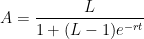
$A = \displaystyle \frac{L}{1 + (L-1)e^{-rt}}$ ,

where $r = \ln 2$ . (Had each person the rumor to two different people at each step, then $r$ would have been equal to $r = \ln 3$ .) Here’s the graph, superimposed upon the data collected from class. I can do this pretty quickly in class because the curve is actually already drawn in the figure above… but it’s drawn in gray, the same color as the background. By changing the color to black, the graph becomes clear:

I never expect the curve to exactly fit the data, but it should come pretty close. After this fairly dramatic revelation, my students are completely sold that the mathematics that I’m about to show them actually works.

Exponential growth and decay (Part 13): Newton’s Law of Cooling

In this series of posts, I provide a deeper look at common applications of exponential functions that arise in an Algebra II or Precalculus class. In the previous posts in this series, I considered financial applications. In today’s post, I’ll discuss Newton’s Law of Cooling, which describes how quickly a hot object cools in a room at constant temperature. (This law is not to be confused with Newton’s Three Laws of Motion.)

While Newton’s Law of Cooling is easy to state, not many high school teachers are aware of the physical principles from which they arise. The basic idea is that the rate at which a hot object cools is proportional to the difference between its current temperature and the surrounding temperature. After solving the appropriate differential equation, the temperature $T(t)$ of the object is found to be

$T = S + (T_0 - S) e^{-kt}$ ,

where $t$ is the time, $S$ is the constant surrounding temperature, and $k$ is a constant that depends on the object.

Of course, students in Algebra II or Precalculus (or high school physics) are usually not ready to understand this derivation using calculus. Instead, they are typically given the final formula and are expected to use this formula to solve problems. Still, I think it’s important for the teacher of Algebra II or Precalculus to be aware of how the origins of this formula, as it only requires mathematics that’s only a year or two away in these students’ mathematical development.

This is the third application of exponential functions considered in this series; the previous two were continuous compound interest and radioactive decay. Unlike these previous two applications, Newton’s Law of Cooling can actually be demonstrated in class to engage students. All that’s required is the appropriate classroom technology and a standard-issue temperature probe.This stands in sharp contrast to the previous applications of exponential functions considered in this series. While students can easily envision making money via compound interest, no one will actually give them the money during class. And certainly I don’t encourage performing a real demonstration of radioactive decay with, say uranium-235, during class time! (There are ways of simulating radioactive decay using M&Ms or other manipulatives, however.)

A simple Google search yields thousands of webpages describes multiple classroom activities for Newton’s Law of Cooling. Some activities merely require collecting data and performing a regression fit to an exponential curve; such an activity would be appropriate for middle-school students. Other activities are more explicit about using Newton’s Law of Cooling. Here’s a sampling:

These links are aimed at a students at a variety of levels. Indeed, it’s possible to use a graphing calculator to plot the numerical derivative $T'(t)$ as a function of time, use linear regression to solve for the constant $k$ , and then produce the exponential curve using this value of $k$ . Several years ago, I saw an effective demonstration of this idea at the Joint Mathematics Meetings in which the presenters covered these aspects of Newton’s Law of Cooling in less than 10 minutes. (Naturally, additional time is needed when students perform these activities for themselves.)

Exponential growth and decay (Part 9): Amortization tables

This post is inspired by one of the questions that I pose to our future high school math teachers during our Friday question-and-answer sessions. In these sessions, I play the role of a middle- or high-school student who’s asking a tricky question to his math teacher. Here’s the question:

A student asks, “My father bought a house for $200,000 at 12% interest. He told me that by the time he finishes paying for the house, it will have cost him more than $500,000. How is that possible? 12% of $200,000 is only $24,000.”

Without fail, these future teachers don’t have a good response to this question. Indeed, my experience is that most young adults (including college students) have never used an amortization table, which is the subject of today’s post.

In the past few posts, we have considered the solution of the following recurrence relation, which is often used to model the payment of a mortgage or of credit-card debt:

$A_{n+1} = r A_n - k$

With this difference equation, the rate at which the principal is reduced can be simply computed using Microsoft Excel. This tool is called an amortization schedule or an amortization table; see E-How for the instructions of how to build one. Here’s a sample Excel spreadsheet that I’ll be illustrating below: Amortization schedule. My personal experience is that many math majors have never seen such a spreadsheet, even though they are familiar with compound interest problems and certainly have the mathematical tools to understand this spreadsheet.

Here’s a screen capture from the spreadsheet:

The terms of the loan are typed into Cells B1 (length of loan, in years), B2 (annual percentage rate), and B3 (initial principal). Cell B4 is computed from this information using the Microsoft Excel command $\hbox{PMT}$ :

$=\hbox{PMT}(\hbox{B2}/12,\hbox{B1}*12,-\hbox{B3})$

This is the amount that must be paid every month in order to pay off the loan in the prescribed number of years. Of course, there is a formula for this:

$M = \displaystyle \frac{Pr}{12 \displaystyle \left[1 - \left( 1 + \frac{r}{12} \right)^{-12t} \right]}$

I won’t go into the derivation of this formula here, as it’s a bit complicated. Notice that this formula does not include escrow, points, closing costs, etc. This is strictly the amount of money that’s needed to pay down the principal.

The table, beginning in Row 8 of the above picture, shows how quickly the principal will be paid off. In row 8, the interest that’s paid for that month is computed by

$=\hbox{B8} * \$ \hbox{B}\$\hbox{2}/12$

Therefore, the amount of the monthly payment that actually goes toward paying down the principal will be

$= \$\hbox{B}\$\hbox{4} - \hbox{C8}$

Column E provides an opportunity to pay something extra each month; more on this later. So, after taking into account the payments in columns D and E, the amount remaining on the loan is recorded in Cell F8:

$= \hbox{B8} - \hbox{D8} - \hbox{E8}$

This amount is then copied into Cell B9, and then the pattern can be filled down.

The yellow graph shows how quickly the balance of the loan is paid off over the length of the loan. A picture is worth a thousand words: in the initial years of the loan, most of the payments are gobbled up by the interest, and so the principal is paid off slowly. Only in the latter years of the loan is the principal paid off quickly.

So, it stands to reason that any extra payments in the initial months and years of the loan can do wonders for paying off the loan quickly. For example, here’s a screenshot of what happens if an extra $200/month is paid only in the first 12 months of the loan:

A definite bend in the graph is evident in the initial 12 months until the normal payment is resumed in month 13. As a result of those extra payments, the curve now intersects the horizontal axis around 340. In other words, 20 fewer months are required to pay off the loan. Stated another way, the extra payments in the first year cost an extra $\$200 \times 12 = \$2400$ . However, in the long run, those payments saved about $\$536.82 \times 20 \approx \$10,700$ !

Exponential growth and decay (Part 8): Paying off credit-card debt via recurrence relations

The following problem in differential equations has a very practical application for anyone who has either (1) taken out a loan to buy a house or a car or (2) is trying to pay off credit card debt. To my surprise, most math majors haven’t thought through the obvious applications of exponential functions as a means of engaging their future students, even though it is directly pertinent to their lives (both the students’ and the teachers’).

You have a balance of $2,000 on your credit card. Interest is compounded continuously with a rate of growth of 25% per year. If you pay the minimum amount of $50 per month (or $600 per year), how long will it take for the balance to be paid?

In previous posts, I approached this problem using differential equations. There’s another way to approach this problem that avoids using calculus that, hypothetically, is within the grasp of talented Precalculus students. Instead of treating this problem as a differential equation, we instead treat it as a first-order difference equation (also called a recurrence relation):

$A_{n+1} = r A_n - k$

The idea is that the amount owed is multiplied by a factor $r$ (which is greater than 1), and from this product the amount paid is deducted. With this approach — and unlike the approach using calculus — the payment period would be each month and not per year. Therefore, we can write

$A_{n+1} = \displaystyle \left( 1 + \frac{0.25}{12} \right) A_n - 50$

Notice that the meaning of the 25% has changed somewhat… it’s no longer the relative rate of growth, as the 25% has been equally divided for the 12 months. The solution of this difference equation is

$A_n = r^n P - k \left( \displaystyle \frac{1 - r^n}{1-r} \right)$

green line

A great advantage of using a difference equation to solve this problem is that the solution can be easily checked with a simple spreadsheet. (Indeed, pedagogically, I would recommend showing a spreadsheet like this before doing any of the calculations of the previous few posts, so that students can begin to wrap their heads around the notion of a difference equation before the solution is presented.)

To start the spreadsheet, I wrote “Step” in Cell A1 and “Amount” in Cell B1. Then I entered the initial conditions: $0$ in Cell A2 and $2000$ in Cell B2. (In the screenshot below, I changed the format of column B to show dollars and cents.) Next, I entered $=\hbox{A2}+1$ in Cell A3 and

$=\hbox{B2}*(1+0.25/12)-50$

in Cell B3. Finally, I copied the pattern in Cells A3 and B3 downward. Here’s the result:

After the formula the algebraic solution of the difference equation has been found, this can be added to the spreadsheet in a different column. For example, I added the header “Predicted Amount” in Cell D1. In Cell D2, I typed the formula

$=2000*\hbox{POWER}(1+0.25/12,\hbox{A2})-50*(1-\hbox{POWER}(1+0.25/12,\hbox{A2}))/(1-(1+0.25/12))$

Finally, I copied this pattern down the Column D. Here’s the result:

Invariably, when I perform a demonstration like this in class, I elicit a reaction of “Whoa…. it actually works!” Even for a class of math majors. Naturally, I tease them about this… they didn’t believe me when I used algebra, but now it has to be true because the computer says so.

Here’s the spreadsheet that I used to make the above pictures: CreditCardDebt.