In my capstone class for future secondary math teachers, I ask my students to come up with ideas for engaging their students with different topics in the secondary mathematics curriculum. In other words, the point of the assignment was not to devise a full-blown lesson plan on this topic. Instead, I asked my students to think about three different ways of getting their students interested in the topic in the first place.
I plan to share some of the best of these ideas on this blog (after asking my students’ permission, of course).
This student submission comes from my former student Alyssa Dalling. Her topic, from Precalculus: the equation of a circle.
A. How could you as a teacher create an activity or project that involves your topic?
A fun way to engage students and also introduce the standard form of an equation of a circle is the following:
Start by separating the class into groups of 2 or 3
Pass each group a specific amount of flashcards. (Each group will have the same flashcards)
Each flashcard has a picture of a graphed circle and the equation of that circle in standard form
The students will work together to figure out how the pictures of the circle relate to the equation
This will help students understand how different aspects of a circle relate to its standard form equation. The following is an example of a flashcard that could be passed out.
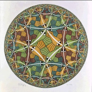
C. How has this topic appeared in high culture (art, classical music, theatre, etc.)?
Circles have been used through history in many different works of art. One such type is called a tessellation. The word Tessellate means to cover a plane with a pattern in such a way as to leave no region uncovered. So, a tessellation is created when a shape or shapes are repeated over and over again. The pictures above show just a few examples of how circles are used in different types of art. A good way to engage students would be to show them a few examples of tessellations using circles.
E. How can technology be used to effectively engage students with this topic?
Khan Academy has a really fun resource for using equations to graph circles. At the beginning of class, the teacher could allow students to play around with this program. It allows students to see an equation of a circle in standard form then they would graph the circle. It gives hints as well as the answer when students are ready. The good thing about this is that even if a student goes straight to the answer, they are still trying to identify the connection between the equation of the circle and the answer Khan Academy shows.
This post is not really about finding square roots but continues Part 8 of this series. Continuing the theme of this series, let’s go back in time to when scientific calculators were not invented… say, 1850.
This is a favorite activity that I use when teaching logarithms to precalculus students. I begin by writing the following on the board, in three or four columns:
In other words, I tell the answer to only and . The challenge: fill in the rest without a calculator.
In my classes, we found these logarithms by large-group discussion. However, there’s no reason why this couldn’t be done by dividing a class into small groups and letting the groups collaborate. Indeed, I suggested this idea to a former student who was struggling to come up with an engaging activity involving logarithms for an Algebra II class that she was about to teach. She took this idea and ran with it, and she told me it was a big hit with her students.
I provide a thought bubble if you’d like to think about it before I give the answers.
Step 1. Three of these values — , , and — can be found exactly since they’re powers of .
Step 2. Most of the others can be found by using the laws of logarithms for products, quotients, and powers involving , , and . For example,
.
Of this group, usually is the hardest for students to recognize.
Step 3 (optional). A few of the logarithms, like , cannot be determined in terms of and . But they can be approximated to reasonable accuracy with a little creativity. For example,
.
For a really good approximation, we use the fact that .
.
To approximate , we could use the fact that , or . So
Naturally, any and all of the above results can be confirmed with a scientific calculator.
In my opinion, here are some of the pedagogical benefits of the above activity.
1. This activity solidifies students’ knowledge about the laws of logarithms. The laws of logarithms become less abstract, changing from into something more tangible and comfortable, like positive integers.
2. Hopefully the activity will demystify for students the curious decimal expansions when a calculator returns logarithms. In other words, hopefully the above activity will help
3. The activity should promote some understanding of the values of base-10 logarithms. For example, for and for .
4. Students should see that, for large , is not much larger than . This is another way of saying that the graph of increases very slowly as increases. So this should provide some future intuition for the graphs of logarithmic functions.
5. The values of are used to construct the unevenly-spaced lines and/or tick marks in log-log graphs and log-linear graphs (which are standard plotting options on many scientific calculators).
I’m in the middle of a series of posts concerning the elementary operation of computing a root. This is such an elementary operation because nearly every calculator has a button, and so students today are accustomed to quickly getting an answer without giving much thought to (1) what the answer means or (2) what magic the calculator uses to find roots. I like to show my future secondary teachers a brief history on this topic… partially to deepen their knowledge about what they likely think is a simple concept, but also to give them a little appreciation for their elders.
To begin, let’s again go back to a time before the advent of pocket calculators… say, 1952.
This story doesn’t go back to 1952 but to Boxing Day 2012 (the day after Christmas). For some reason, my daughter — out of the blue — asked me to compute without a calculator. As my daughter adores the ground I walk on — and I want to maintain this state of mind for as long as humanly possible — I had no choice but to comply. So I might as well have been back in 1952.
In the past few posts, I discussed how log tables and slide rules were used by previous generations to perform this calculation. The problem was that all of these tools were in my office and not at home, and hence were not of immediate use.
The good news is that I had a few logarithms memorized:
, , ,
and .
I had the first two logs memorized when I was a child; the third I memorized later. As I’ll describe, the first three logarithms can be used with the laws of logarithms to closely approximate the base-10 logarithm of nearly any number. The last logarithm was important in previous generations for using the change-of-base formula from to . It was also prominently mentioned in the chapter “Lucky Numbers” from a favorite book of my childhood, Surely You’re Joking Mr. Feynman, so I had that memorized as well.
To begin, I first noticed that , and I knew I could get since . So I started with
I did all of the above calculations by hand, cutting off after three decimal places (since I had those base-10 logarithms memorized to only three decimal places). Therefore,
So, to complete the calculation, I had to find the value of so that . This was by far the hardest step, since it could only be done by trial and error. I forget exactly what steps I tried, but here’s a sample:
. Too big.
. Too small.
. Too small.
. Too big.
Eventually, I got to
So, after a hour or two of arithmetic, I told her my answer: . You can imagine my sheer delight when we checked my answer with a calculator:
In Part 9, I’ll discuss my opinion about whether or not these kinds of calculations have any pedagogical value for students learning logarithms.
I’m in the middle of a series of posts concerning the elementary operation of computing a square root. This is such an elementary operation because nearly every calculator has a button, and so students today are accustomed to quickly getting an answer without giving much thought to (1) what the answer means or (2) what magic the calculator uses to find square roots. I like to show my future secondary teachers a brief history on this topic… partially to deepen their knowledge about what they likely think is a simple concept, but also to give them a little appreciation for their elders.
Today’s topic — slide rules — not only applies to square roots but also multiplication, division, and raising numbers to any exponent (not just to the power). To begin, let’s again go back to a time before the advent of pocket calculators… say, the 1950s.
Nearly all STEM professionals were once proficient in the use of slide rules. I never learned how to use one as a student. As a college professor, I bought a fairly inexpensive one from Slide Rule Universe. If you’ve never seen a slide rule, here’s a picture of a fairly advanced one. There are multiple rows of numbers and a sliding plastic piece that has a thin vertical line, allowing direct correspondence from one row of numbers to another. (The middle rows are on a piece that slides back and forth; this is necessary for doing multiplication and division with a slide rule.)
Let’s repeat the problem from Part 6 and try to find
.
We recall that . The logarithm on the right-hand side can be estimated by looking at a slide rule. Here’s a picture from my slide rule:
The important parts of this picture are the bottom two rows. Note that the thin red line is lined up between and ; indeed, the red line is about one-third of way from to . On the bottom row, the thin red line is lined up with . So we estimate that , so that .
Working the other direction, we must find . We move the thin red line to a different part of the slide rule:
This time, the thin red line is lined up with on the bottom row. On the row above, the red line is lined up almost exactly on , but perhaps a little to the left of . So we estimate that or .
The correct answer is .
Not bad for a piece of plastic.
Because taking square roots is so important, many slide rules have lines that simulate a square-root function… without the intermediate step of taking logarithms. Let’s consider again at the above picture, but this time let’s look at the second row from the top. Notice that the thin red line goes between and on the second line. (FYI, the line repeats itself to the left, so that the user can tell the difference between and .) Then looking down to the second line from the bottom, we see that the square root is a little less than , as before.
In addition to square roots, my personal slide rule has lines for cube roots, sines, cosines, and tangents. In the past, more expensive slide rules had additional lines for the values of other mathematical functions.
More thoughts on slide rules:
1. Slide rules can be used for multiplication and division; the Slide Rule University website also a good explanation for how this works.
2. In a fairly modern film, Apollo 13 (released in 1995 but set in 1970), engineers using slide rules were shown to dramatic effect.
3. Slide rule apps can be downloaded onto both iPhones and Android smartphones; here’s the one that I use. I personally take great anachronistic pleasure in using a slide rule app on my smartphone.
4. While slide rules have been supplanted by scientific calculators, I do believe that slide rules still have modern pedagogical value. I’ve had many friends tell me that, when they were in school, they were asked to construct their own slide rules from scratch (though not as detailed as professional slide rules). I think this would be a reasonable exploration activity that can still engage today’s students (as well as give them some appreciation for their elders).
I’m in the middle of a series of posts concerning the elementary operation of computing a square root. This is such an elementary operation because nearly every calculator has a button, and so students today are accustomed to quickly getting an answer without giving much thought to (1) what the answer means or (2) what magic the calculator uses to find square roots. I like to show my future secondary teachers a brief history on this topic… partially to deepen their knowledge about what they likely think is a simple concept, but also to give them a little appreciation for their elders.
In Parts 3-5 of this series, I discussed how log tables were used in previous generations to compute logarithms and antilogarithms.
Today’s topic — log tables — not only applies to square roots but also multiplication, division, and raising numbers to any exponent (not just to the power). After showing how log tables were used in the past, I’ll conclude with some thoughts about its effectiveness for teaching students logarithms for the first time.
To begin, let’s again go back to a time before the advent of pocket calculators… say, the 1880s.
Aside from a love of the movies of both Jimmy Stewart and John Wayne, I chose the 1880s on purpose. By the end of that decade, James Buchanan Eads had built a bridge over the Mississippi River and had designed a jetty system that allowed year-round navigation on the Mississippi River. Construction had begun on the Panama Canal. In New York, the Brooklyn Bridge (then the longest suspension bridge in the world) was open for business. And the newly dedicated Statue of Liberty was welcoming American immigrants to Ellis Island.
And these feats of engineering were accomplished without the use of pocket calculators.
Here’s a perfectly respectable way that someone in the 1880s could have computed to reasonably high precision. Let’s write
.
Take the base-10 logarithm of both sides.
.
Then log tables can be used to compute .
Step 1. In our case, we’re trying to find . We know that and , so the answer must be between and . More precisely,
.
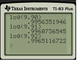
To find , we see from the table that
and
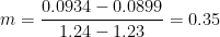
So, to estimate , we will employ linear interpolation. That’s a fancy way of saying “Find the line connecting and , and find the point on the line whose coordinate is . Finding this line is a straightforward exercise in the point-slope form of a line:
So we estimate . Thus, so far in the calculation, we have
Step 2. We then take the antilogarithm of both sides. The term antilogarithm isn’t used much anymore, but the principle is still taught in schools: take to the power of both the left- and right-hand sides. We obtain
The first part of the right-hand side is easy: . For the second-part, we use the log table again, but in reverse. We try to find the numbers that are closest to in the body of the table. In our case, we find that
and .
Once again, we use linear interpolation to find the line connecting and , except this time the coordinate of is known and the coordinate is unknown.
Since the table is only accurate to four significant digits, we estimate that . Therefore,
By way of comparison, the answer is , rounding at the hundredths digit. Not bad, for a generation born before the advent of calculators.
With a little practice, one can do the above calculations with relative ease. Also, many log tables of the past had a column called “proportional parts” that essentially replaced the step of linear interpolation, thus speeding the use of the table considerably.
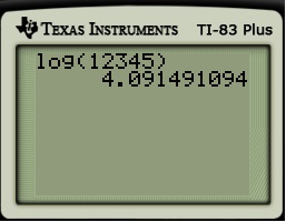
Log tables can be used for calculations more complex than finding a square root. For example, suppose I need to calculate
Using the log table, and without using a calculator, I find that
That’s the correct answer to four significant digits. Using a calculator, we find the answer is
I’m in the middle of a series of posts concerning the elementary operation of computing a square root. This is such an elementary operation because nearly every calculator has a button, and so students today are accustomed to quickly getting an answer without giving much thought to (1) what the answer means or (2) what magic the calculator uses to find square roots. I like to show my future secondary teachers a brief history on this topic… partially to deepen their knowledge about what they likely think is a simple concept, but also to give them a little appreciation for their elders.
One way that square roots can be computed without a calculator is by using log tables. This was a common computational device before pocket scientific calculators were commonly affordable… say, the 1920s.
As many readers may be unfamiliar with this blast from the past, Parts 3 and 4 of this series discussed the mechanics of how to use a log table. In Part 6, I’ll discuss how square roots (and other operations) can be computed with using log tables.
In this post, I consider the modern pedagogical usefulness of log tables, even if logarithms can be computed more easily with scientific calculators.
A personal story: In either 1981 or 1982, my parents bought me my first scientific calculator. It was a thing of beauty… maybe about 25% larger than today’s TI-83s, with an LED screen that tilted upward. When it calculated something like , the screen would go blank for a couple of seconds as it struggled to calculate the answer. I’m surprised that smoke didn’t come out of both sides as it struggled. It must have cost my parents a small fortune, maybe over $1000 after adjusting for inflation. Naturally, being an irresponsible kid in the early 1980s, it didn’t last but a couple of years. (It’s a wonder that my parents didn’t kill me when I broke it.)
So I imagine that requiring all students to use log tables fell out of favor at some point during the 1980s, as technology improved and the prices of scientific calculators became more reasonable.
I regularly teach the use of log tables to senior math majors who aspire to become secondary math teachers. These students who have taken three semesters of calculus, linear algebra, and several courses emphasizing rigorous theorem proving. In other words, they’re no dummies. But when I show this blast from the past to them, they often find the use of a log table to be absolutely mystifying, even though it relies on principles — the laws of logarithms and the point-slope form of a line — that they think they’ve mastered.
So why do really smart students, who after all are math majors about to graduate from college, struggle with mastering log tables, a concept that was expected of 15- and 16-year-olds a generation ago? I personally think that a lot of their struggles come from the fact that they don’t really know logarithms in the way that students of previous generation had to know them in order to survive precalculus. For today’s students, a logarithm is computed so easily that, when my math majors were in high school, they were not expected to really think about its meaning.
For example, it’s no longer automatic for today’s math majors to realize that has to be between and someplace. They’ll just punch the numbers in the calculators to get an answer, and the process happens so quickly that the answer loses its meaning.
They know by heart that and that . But it doesn’t reflexively occur to them that these laws can be used to rewrite as .
When encountering , their first thought is to plug into a calculator to get the answer, not to reflect and realize that the answer, whatever it is, has to be between and someplace.
Today’s math majors can be taught these approximation principles, of course, but there’s unfortunately no reason to expect that they received the same training with logarithms that students received a generation ago. So none of this discussion should be considered as criticism of today’s math majors; it’s merely an observation about the training that they received as younger students versus the training that previous generations received.
So, do I think that all students today should exclusively learn how to use log tables? Absolutely not.If college students who have received excellent mathematical training can be daunted by log tables, you can imagine how the high school students of generations past must have felt — especially the high school students who were not particularly predisposed to math in the first place.
People like me that made it through the math education system of the 1980s (and before) received great insight into the meaning of logarithms. However, a lot of students back then found these tables as mystifying as today’s college students, and perhaps they did not survive the system because they found the use of the table to be exceedingly complex. In other words, while they were necessary for an era that pre-dated pocket calculators, log tables (and trig tables) were an unfortunate conceptual roadblock to a lot of students who might have had a chance at majoring in a STEM field. By contrast, logarithms are found easily today so that the steps above are not a hindrance to today’s students.
That said, I do argue that there is pedagogical value (as well as historical value) in showing students how to use log tables, even though calculators can accomplish this task much quicker. In other words, I wouldn’t expect students to master the art of performing the above steps to compute logarithms on the homework assignments and exams. But if they can’t perform the above steps, then there’s room for their knowledge of logarithms to grow.
And it will hopefully give today’s students a little more respect for their elders.
I’m in the middle of a series of posts concerning the elementary operation of computing a square root. In Part 3 of this series, I discussed how previous generations computed logarithms without a calculator by using log tables. In this post, I’ll discuss how previous generations computed, using the language of the time, antilogarithms. In Part 5, I’ll discuss my opinions about the pedagogical usefulness of log tables, even if logarithms can be computed more easily with scientific calculators. And in Part 6, I’ll return to square roots — specifically, how log tables can be used to find square roots.
Let’s again go back to a time before the advent of pocket calculators… say, 1943.
The following log tables come from one of my prized possessions: College Mathematics, by Kaj L. Nielsen (Barnes & Noble, New York, 1958).
How to use the table, Part 5. The table can also be used to work backwards and find an antilogarithm. The term antilogarithm isn’t used much anymore, but the principle is still used in teaching students today. Suppose we wish to solve
, or .
Looking through the body of the table, we see that appears on the row marked and the column marked . Therefore, $10^{0.9509} \approx 8.93$. Again, this matches (to three and almost four significant digits) the result of a modern calculator.
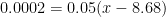
How to use the table, Part 6. Linear interpolation can also be used to find antilogarithms. Suppose we’re trying to evaluate , or find the value of so that $\log_{10} x = 0.9387$. From the table, we can trap between
and
So we again use linear interpolation, except this time the value of is known and the value of is unknown:
So we estimate This matches the result of a modern calculator to four significant digits:
How to use the table, Part 7.
How to use the table, Part 8.
Note: Sorry, but I’m not sure what happened… when the post came up this morning (August 4), I saw my work in Parts 7 and 8 had disappeared. Maybe one of these days I’ll restore this.
I’m in the middle of a series of posts concerning the elementary operation of computing a square root. This is such an elementary operation because nearly every calculator has a button, and so students today are accustomed to quickly getting an answer without giving much thought to (1) what the answer means or (2) what magic the calculator uses to find square roots. I like to show my future secondary teachers a brief history on this topic… partially to deepen their knowledge about what they likely think is a simple concept, but also to give them a little appreciation for their elders.
Today’s topic is the use of log tables. I’m guessing that many readers have either forgotten how to use a log table or else were never even taught how to use them. After showing how log tables were used in the past, I’ll conclude with some thoughts about its effectiveness for teaching students logarithms for the first time.
This will be a fairly long post about log tables. In the next post, I’ll discuss how log tables can be used to compute square roots.
To begin, let’s again go back to a time before the advent of pocket calculators… say, 1912.
Before the advent of pocket calculators, most professional scientists and engineers had mathematical tables for keeping the values of logarithms, trigonometric functions, and the like. The following images come from one of my prized possessions: College Mathematics, by Kaj L. Nielsen (Barnes & Noble, New York, 1958). Some saint gave this book to me as a child in the late 1970s; trust me, it was well-worn by the time I actually got to college.
With the advent of cheap pocket calculators, mathematical tables are a relic of the past. The only place that any kind of mathematical table common appears in modern use are in statistics textbooks for providing areas and critical values of the normal distribution, the Student distribution, and the like.
That said, mathematical tables are not a relic of the remote past. When I was learning logarithms and trigonometric functions at school in the early 1980s — one generation ago — I distinctly remember that my school textbook had these tables in the back of the book.
And it’s my firm opinion that, as an exercise in history, log tables can still be used today to deepen students’ facility with logarithms. In this post and Part 4 of this series, I discuss how the log table can be used to compute logarithms and (using the language of past generations) antilogarithms without a calculator. In Part 5, I’ll discuss my opinions about the pedagogical usefulness of log tables, even if logarithms can be computed more easily nowadays with scientific calculators. In Part 6, I’ll return to square roots — specifically, how log tables can be used to find square roots.
How to use the table, Part 1. How do you read this table? The left-most column shows the ones digit and the tenths digit, while the top row shows the hundredths digit. So, for example, the bottom row shows ten different base-10 logarithms:
So, rather than punching numbers into a calculator, the table was used to find these logarithms. You’ll notice that these values match, to four decimal places, the values found on a modern calculator.
How to use the table, Part 2. What if we’re trying to take the logarithm of a number between and which has more than two digits after the decimal point, like ? From the table, we know that the value has to lie between
and
So, to estimate , we will employ linear interpolation. That’s a fancy way of saying “Find the line connecting and , and find the point on the line whose coordinate is . The graph of $y = \log_{10} x$ is not a straight line, of course, but hopefully this linear interpolation will be reasonably close to the correct answer.
Finding this line is a straightforward exercise in the point-slope form of a line:
Remembering that this log table is only good to four significant digits, we estimate .
With a little practice, one can do the above calculations with relative ease. Also, many log tables of the past had a column called “proportional parts” that essentially replaced the step of linear interpolation, thus speeding the use of the table considerably.
Again, this matches the result of a modern calculator to four decimal places:
How to use the table, Part 3. So far, we’ve discussed taking the logarithms of numbers between and and the antilogarithms of numbers between and . Let’s now consider what happens if we pick a number outside of these intervals.
To find , we observe that
More intuitively, we know that the answer must lie between and , so the answer must be . The value of is the necessary .
We then find by linear interpolation. From the table, we see that
and
Employing linear interpolation, we find
Remembering that this log table is only good to four significant digits, we estimate , so that .
Again, this matches the result of a modern calculator to four decimal places (in this case, five significant digits):
How to use the table, Part 4. Let’s now consider what happens if we pick a positive number less than . To find , we observe that
We have already found by linear interpolation. We therefore conclude that . Again, this matches the result of a modern calculator to four decimal places (in this case, five significant digits):
So that’s how to compute logarithms without a calculator: we rely on somebody else’s hard work to compute these logarithms (which were found in the back of every precalculus textbook a generation ago), and we make clever use of the laws of logarithms and linear interpolation.
Log tables are of course subject to roundoff errors. (For that matter, so are pocket calculators, but the roundoff happens so deep in the decimal expansion — the 12th or 13th digit — that students hardly ever notice the roundoff error and thus can develop the unfortunate habit of thinking that the result of a calculator is always exactly correct.)
For a two-page table found in a student’s textbook, the results were typically accurate to four significant digits. Professional engineers and scientists, however, needed more accuracy than that, and so they had entire books of tables. A table showing 5 places of accuracy would require about 20 printed pages, while a table showing 6 places of accuracy requires about 200 printed pages. Indeed, if you go to the old and dusty books of any decent university library, you should be able to find these old books of mathematical tables.
In other words, that’s how the Brooklyn Bridge got built in an era before pocket calculators.
At this point you may be asking, “OK, I don’t need to use a calculator to use a log table. But let’s back up a step. How were the values in the log table computed without a calculator?” That’s a perfectly reasonable question, but this post is getting long enough as it is. Perhaps I’ll address this issue in a future post.
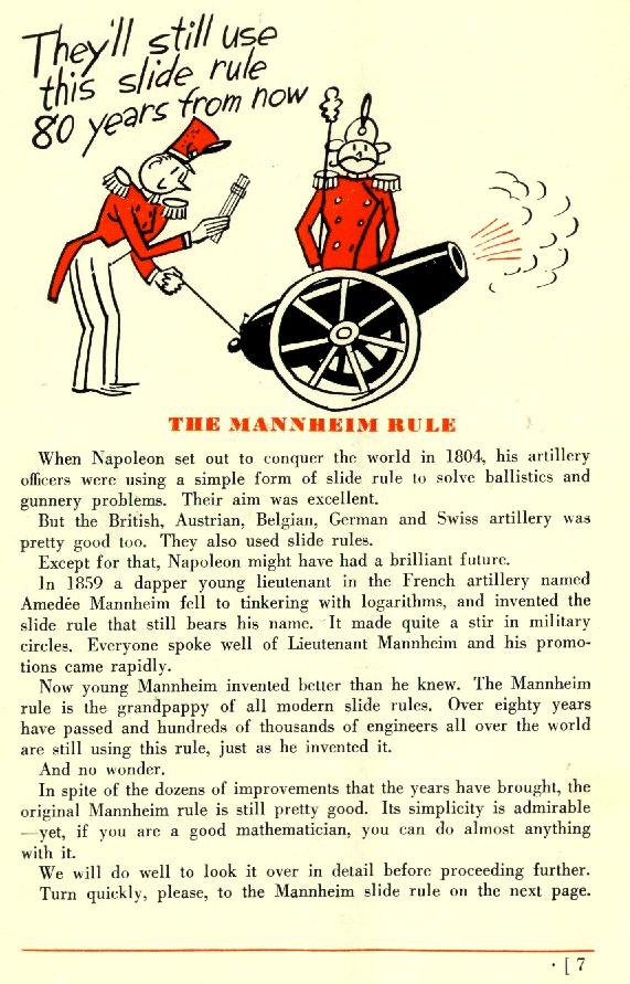
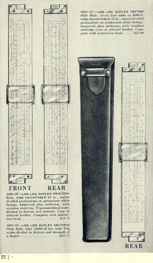
I’m about to begin a series of posts concerning how previous generations did complex mathematical calculations without the aid of scientific calculators.
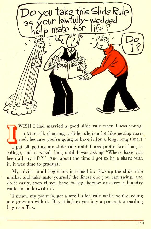
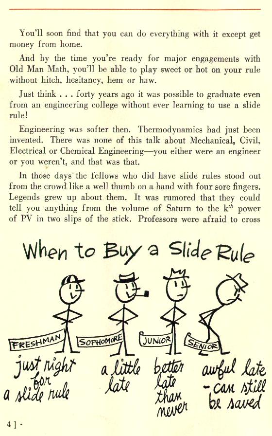
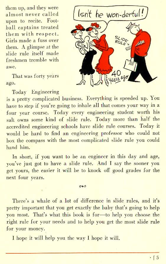
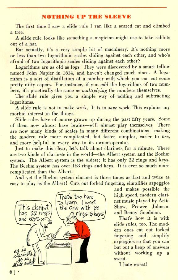
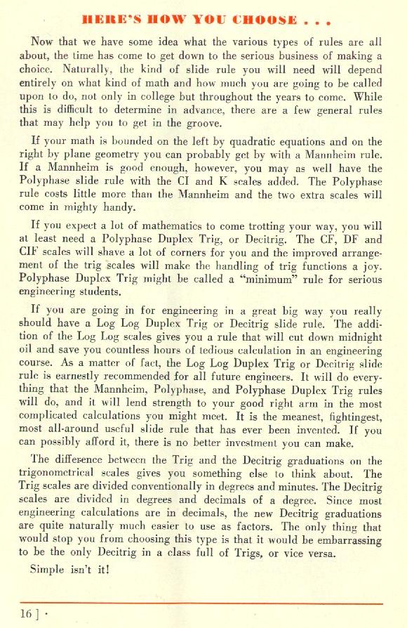
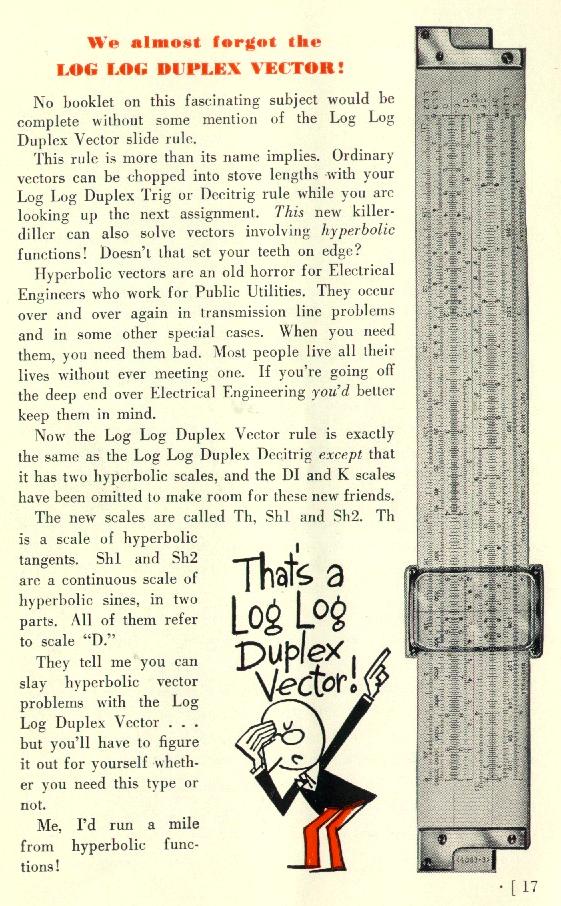
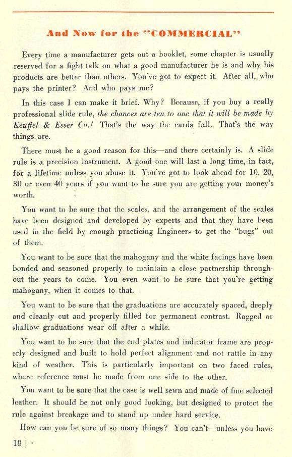
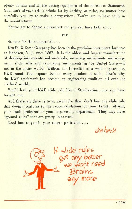
Courtesy of Slide Rule Universe, here’s an advertisement for slide rules from 1940. This is a favorite engagement activity of mine when teaching precalculus (as an application of logarithms) as well as my capstone class for future high school math teachers. I have shown this to hundreds of college students over the years (usually reading out loud the advertising through page 5 and then skimming through the remaining pictures), and this always gets a great laugh. Enjoy.
In my capstone class for future secondary math teachers, I ask my students to come up with ideas for engaging their students with different topics in the secondary mathematics curriculum. In other words, the point of the assignment was not to devise a full-blown lesson plan on this topic. Instead, I asked my students to think about three different ways of getting their students interested in the topic in the first place.
I plan to share some of the best of these ideas on this blog (after asking my students’ permission, of course).
This student submission again comes from my former student Caitlin Kirk. Her topic: how to engage Algebra II or Precalculus students when solving logarithmic equations.
B. Curriculum: How does this topic extend what your students should have learned in previous courses?
Logarithms are a topic that appears at multiple levels of high school math. In Algebra II, students are first introduced to logarithms when they are asked to identify graphs of parent functions including f (x) = logax. Later in the same class, they learn to formulate equations and inequalities based on logarithmic functions by exploring the relationship between logarithms and their inverses. From there, they can develop a definition of a logarithm.
Solving logarithmic equations extends what students learned about logarithms in Algebra II. Once a proper definition of logarithms has been established, along with a graphical foundation of logs, students learn to solve logarithmic equations. Properties of logarithms are used to expand, condense, and solve logarithms without a calculator in Pre Calculus. Practical applications of the logarithmic equation also follow from previous skills. Students learn to calculate the pH of a solution, decibel voltage gain, intensity of earthquakes measure on the Richter scale, depreciation, and the apparent loudness of sound using logarithms.
C. Culture: How has this topic appeared in the news?
One application of logarithmic equations is calculating the intensity of earthquakes measured on the Richter scale using the following equation:
where is the amplitude of the tremor measured in micrometers and is the period of the tremor (time of one oscillation of the earth’s surface) measured in seconds.
Reports of earthquake activity appear in the news often and are always accompanied by a measurement from the Richter scale. One such report can be found here: http://www.bbc.co.uk/news/world-asia-20638696. As the story says, a 7.3 magnitude earthquake struck off the coast of Japan in December of 2012, and created a small tsunami. There were six aftershocks of this quake whose Richter scale measurements are also given. The article also explains how Japan has been able to enact an early warning system that predicts the intensity of an earthquake before it causes damage. All of the calculations given in this story, and almost all others involving earthquakes, involves the use of the Richter scale logarithmic equation.
D. History: What are the contributions of various cultures to this topic?
The development of logarithms saw contributions from several different countries beginning with the Babylonians (2000-1600 BC) who developed the first known mathematical tables. They also introduced square multiplication in which they simply but accurately multiplied two numbers using only addition and subtraction. Michael Stifel, of Germany, was the first mathematician to use an exponent in 1544. He developed an early version of the logarithmic table containing integers and powers of 2. Perhaps the most important contribution to logarithms came from John Napier in Scotland in 1619. He, like the Babylonians, was working with on breaking multiplication, division, and root extraction down to only addition and subtraction. Therefore, he created the “logarithm” of a number defined as follows:
for which he wrote .
Napier’s definition of the logarithm led to the following logarithmic identities that are still taught today:
Henry Briggs, in England, published his work on logarithms in 1624, which included logarithms of 30,000 natural numbers to the 14th decimal place worked by hand! Shortly after, back in Germany, Johannes Kepler used a logarithmic scale on a Cartesian plane to create a linear graph the elliptical shape of the cosmos. In 1632, in Italy, Bonaventura Cavalieri published extensive tables of logarithms including the logs of trig functions (excluding cosine). Finally, Leonhard Euler made one of the most commonly known contributions to logarithms by making the number the base of the natural logarithm (which was also developed by Napier). While it is untrue, as is commonly believed, that Euler invented the number , he did give it the name . He was interested in the number because he wanted to calculate the amount that would result from continually compounded interested on a sum of money and the number kept appearing as a constant in his equation. Therefore he tied to the natural logarithm that was not as widely used because it did not have a base.
Logarithms were developed as a result of the contributions of many cultures spanning Europe and beyond, dating back over 4000 years.


 and
and  . The challenge: fill in the rest without a calculator.
 ,
,  , and
, and  — can be found exactly since they’re powers of
  ,
,  , and
, and 

 .
. .
. .
. .
. , or
, or  . So
. So
 into something more tangible and comfortable, like positive integers.
 for
for  and
and  for
for  .
. ,
,  is not much larger than
  . This is another way of saying that the graph of
  increases very slowly as
  are used to construct the unevenly-spaced lines and/or tick marks in
  button, and so students today are accustomed to quickly getting an answer without giving much thought to (1) what the answer means or (2) what magic the calculator uses to find roots. I like to show my future secondary teachers a brief history on this topic… partially to deepen their knowledge about what they likely think is a simple concept, but also to give them a little appreciation for their elders.
![\sqrt[19]{25727}](https://s0.wp.com/latex.php?latex=%5Csqrt%5B19%5D%7B25727%7D&bg=ffffff&fg=000000&s=0&c=20201002) without a calculator. As my daughter adores the ground I walk on — and I want to maintain this state of mind for as long as humanly possible — I had no choice but to comply. So I might as well have been back in 1952.
without a calculator. As my daughter adores the ground I walk on — and I want to maintain this state of mind for as long as humanly possible — I had no choice but to comply. So I might as well have been back in 1952. ,
, .
. to
to  . It was also prominently mentioned in the chapter “Lucky Numbers” from a favorite book of my childhood,
  for
for  from the
  .
. , and I knew I could get
  since
since  . So I started with


 . This was by far the hardest step, since it could only be done by trial and error. I forget exactly what steps I tried, but here’s a sample:
 . Too small.
 . Too small.
 . Too big.


![\sqrt[19]{25727} \approx 1.71](https://s0.wp.com/latex.php?latex=%5Csqrt%5B19%5D%7B25727%7D+%5Capprox+1.71&bg=ffffff&fg=000000&s=0&c=20201002) . You can imagine my sheer delight when we checked my answer with a calculator:
. You can imagine my sheer delight when we checked my answer with a calculator: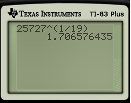
 power). To begin, let’s again go back to a time before the advent of pocket calculators… say, the 1950s.
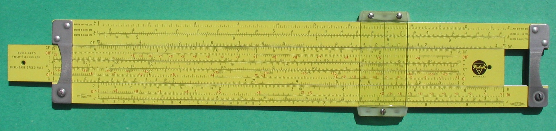
 .
. . The logarithm on the right-hand side can be estimated by looking at a slide rule. Here’s a picture from my slide rule:
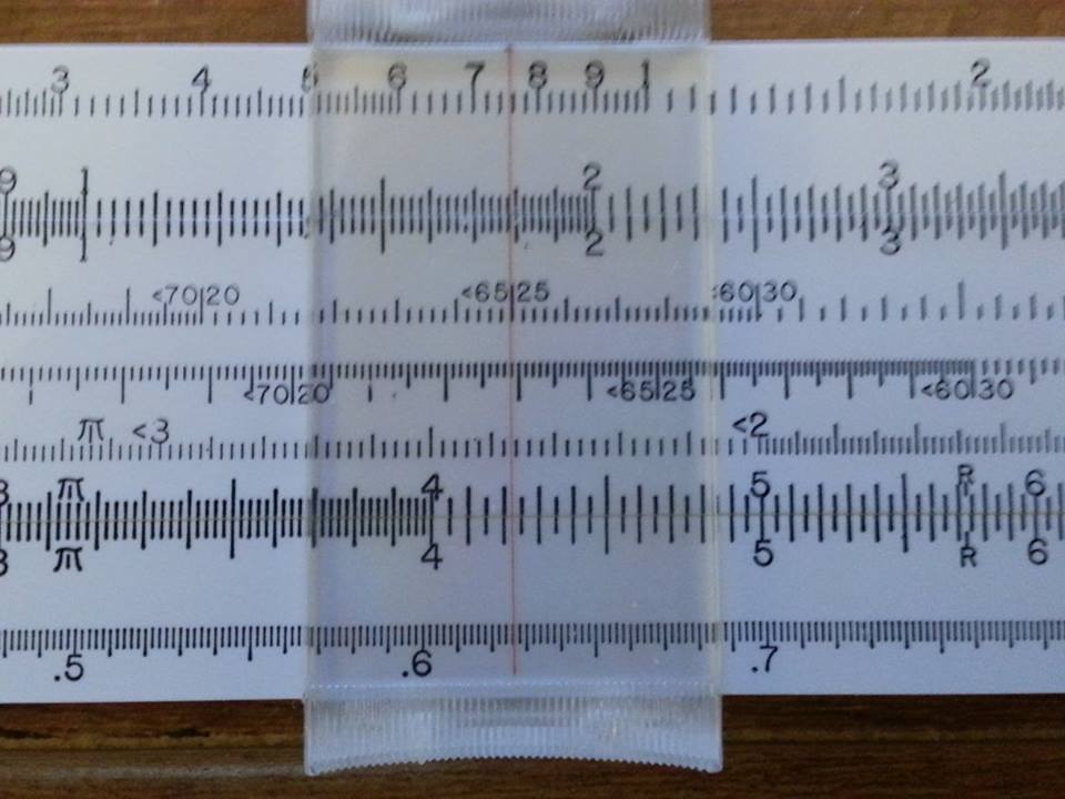
 and
and  ; indeed, the red line is about one-third of way from
  . So we estimate that
  , so that
  .
. . We move the thin red line to a different part of the slide rule:
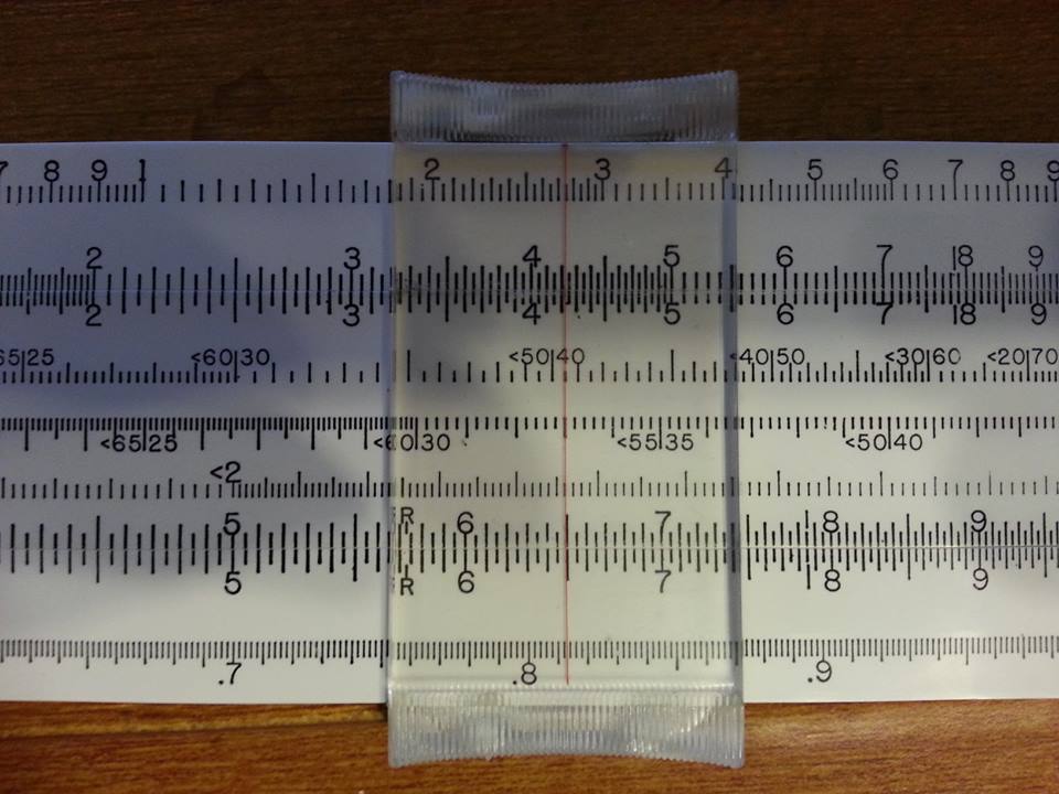
 on the bottom row. On the row above, the red line is lined up almost exactly on
  , but perhaps a little to the left of
  or
or  .
. .
. and
and  on the second line. (FYI, the line repeats itself to the left, so that the user can tell the difference between
  , as before.
 to reasonably high precision. Let’s write
 .
. .
.

 and
and  , so the answer must be between
  . More precisely,
 .
. , we see from the table that
 and
and 
 and
and  , and find the point on the line whose
  coordinate is
  . Finding this line is a straightforward exercise in the
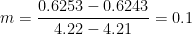


 . Thus, so far in the calculation, we have

 . For the second-part, we use the log table again, but in reverse. We try to find the numbers that are closest to
  in the body of the table. In our case, we find that
 and
and  .
. and
and  , except this time the
  coordinate of
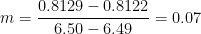


 . Therefore,
 , rounding at the hundredths digit. Not bad, for a generation born before the advent of calculators.


 and that
  . But it doesn’t reflexively occur to them that these laws can be used to rewrite
  .
. , their first thought is to plug into a calculator to get the answer, not to reflect and realize that the answer, whatever it is, has to be between
  , or
, or  .
. appears on the row marked
  and the column marked
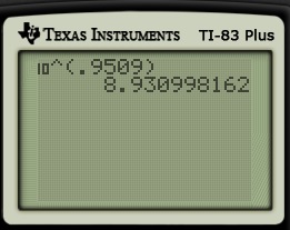
 , or find the value of
  between
 and
and 
 is known and the value of


 This matches the result of a modern calculator to four significant digits:
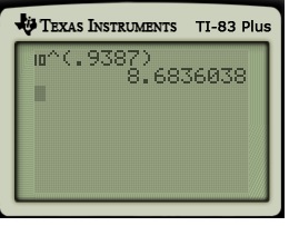
 distribution, and the like.


 ? From the table, we know that the value has to lie between
 and
and 
 and
and  , and find the point on the line whose
  . The graph of $y = \log_{10} x$ is not a straight line, of course, but hopefully this linear interpolation will be reasonably close to the correct answer.


 .
.
 and
and  , we observe that


 , so the answer must be
  . The value of
  is the necessary
  .
. and
and 


 , so that
  .
.
 , we observe that


 . Again, this matches the result of a modern calculator to four decimal places (in this case, five significant digits):


 is the amplitude of the tremor measured in micrometers and
  is the period of the tremor (time of one oscillation of the earth’s surface) measured in seconds.
 of a number
  defined as follows:
 .
.


 the base of the natural logarithm (which was also developed by Napier). While it is untrue, as is commonly believed, that Euler invented the number
  , he did give it the name
  . He was interested in the number because he wanted to calculate the amount that would result from continually compounded interested on a sum of money and the number