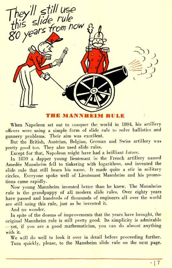
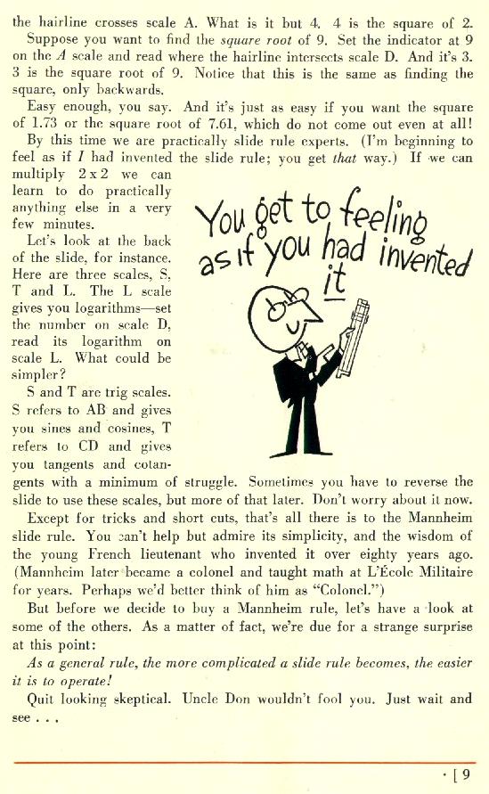
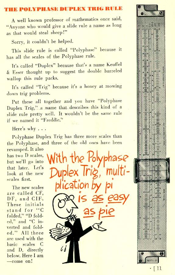
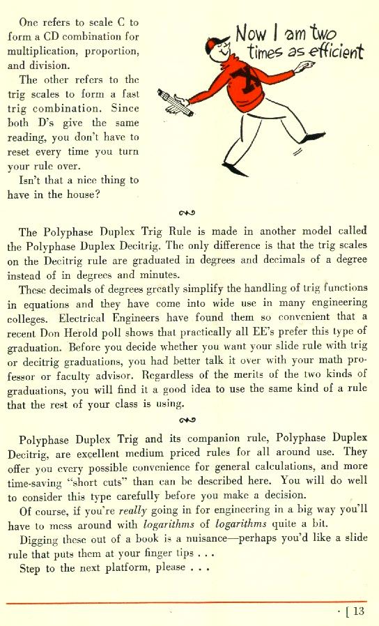
Advertising for slide rules, from 1940

I’m about to begin a series of posts concerning how previous generations did complex mathematical calculations without the aid of scientific calculators.

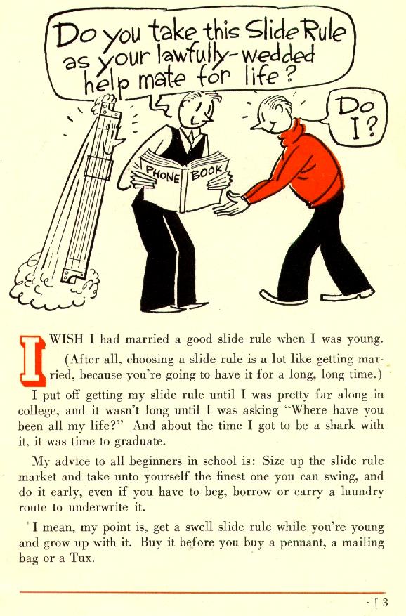
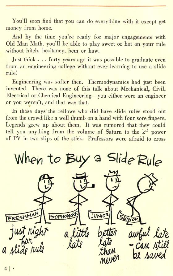
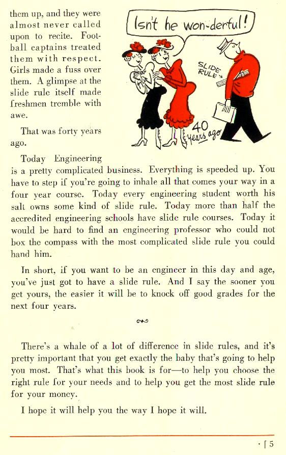
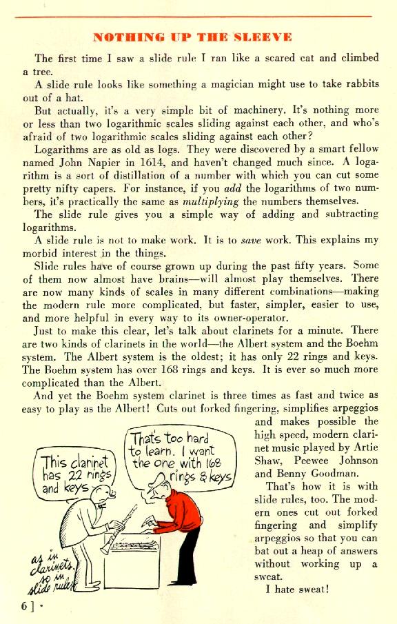
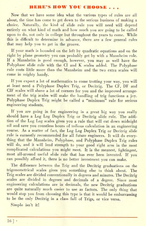
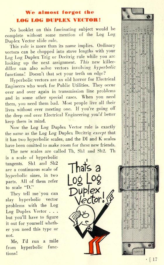
Courtesy of Slide Rule Universe, here’s an advertisement for slide rules from 1940. This is a favorite engagement activity of mine when teaching precalculus (as an application of logarithms) as well as my capstone class for future high school math teachers. I have shown this to hundreds of college students over the years (usually reading out loud the advertising through page 5 and then skimming through the remaining pictures), and this always gets a great laugh. Enjoy.

test

Engaging students: Solving logarithmic equations

In my capstone class for future secondary math teachers, I ask my students to come up with ideas for engaging their students with different topics in the secondary mathematics curriculum. In other words, the point of the assignment was not to devise a full-blown lesson plan on this topic. Instead, I asked my students to think about three different ways of getting their students interested in the topic in the first place.

I plan to share some of the best of these ideas on this blog (after asking my students’ permission, of course).

This student submission again comes from my former student Caitlin Kirk. Her topic: how to engage Algebra II or Precalculus students when solving logarithmic equations.

B. Curriculum: How does this topic extend what your students should have learned in previous courses?

Logarithms are a topic that appears at multiple levels of high school math. In Algebra II, students are first introduced to logarithms when they are asked to identify graphs of parent functions including f (x) = log_ax. Later in the same class, they learn to formulate equations and inequalities based on logarithmic functions by exploring the relationship between logarithms and their inverses. From there, they can develop a definition of a logarithm.

Solving logarithmic equations extends what students learned about logarithms in Algebra II. Once a proper definition of logarithms has been established, along with a graphical foundation of logs, students learn to solve logarithmic equations. Properties of logarithms are used to expand, condense, and solve logarithms without a calculator in Pre Calculus. Practical applications of the logarithmic equation also follow from previous skills. Students learn to calculate the pH of a solution, decibel voltage gain, intensity of earthquakes measure on the Richter scale, depreciation, and the apparent loudness of sound using logarithms.

C. Culture: How has this topic appeared in the news?

One application of logarithmic equations is calculating the intensity of earthquakes measured on the Richter scale using the following equation:

$R = \log(A/P)$

where $A$ is the amplitude of the tremor measured in micrometers and $P$ is the period of the tremor (time of one oscillation of the earth’s surface) measured in seconds.

Reports of earthquake activity appear in the news often and are always accompanied by a measurement from the Richter scale. One such report can be found here: http://www.bbc.co.uk/news/world-asia-20638696. As the story says, a 7.3 magnitude earthquake struck off the coast of Japan in December of 2012, and created a small tsunami. There were six aftershocks of this quake whose Richter scale measurements are also given. The article also explains how Japan has been able to enact an early warning system that predicts the intensity of an earthquake before it causes damage. All of the calculations given in this story, and almost all others involving earthquakes, involves the use of the Richter scale logarithmic equation.

D. History: What are the contributions of various cultures to this topic?

The development of logarithms saw contributions from several different countries beginning with the Babylonians (2000-1600 BC) who developed the first known mathematical tables. They also introduced square multiplication in which they simply but accurately multiplied two numbers using only addition and subtraction. Michael Stifel, of Germany, was the first mathematician to use an exponent in 1544. He developed an early version of the logarithmic table containing integers and powers of 2. Perhaps the most important contribution to logarithms came from John Napier in Scotland in 1619. He, like the Babylonians, was working with on breaking multiplication, division, and root extraction down to only addition and subtraction. Therefore, he created the “logarithm” $L$ of a number $N$ defined as follows:

$N = 10^7 (1-10^{-7})^L$

for which he wrote $\hbox{NapLog}(N) = L$ .

Napier’s definition of the logarithm led to the following logarithmic identities that are still taught today:

$\hbox{NapLog}(\sqrt{N_1N_2}) = \frac{1}{2} (\hbox{NapLog} N_1 + \hbox{NapLog} N_2)$

$\hbox{NapLog}(10^{-7} N_1 N_2) = \hbox{NapLog} N_1 + \hbox{NapLog} N_2$

$\hbox{NapLog} \left( 10^{-7} \displaystyle \frac{N_1}{N_2} \right)= \hbox{NapLog} N_1 - \hbox{NapLog} N_2$

Henry Briggs, in England, published his work on logarithms in 1624, which included logarithms of 30,000 natural numbers to the 14th decimal place worked by hand! Shortly after, back in Germany, Johannes Kepler used a logarithmic scale on a Cartesian plane to create a linear graph the elliptical shape of the cosmos. In 1632, in Italy, Bonaventura Cavalieri published extensive tables of logarithms including the logs of trig functions (excluding cosine). Finally, Leonhard Euler made one of the most commonly known contributions to logarithms by making the number $e = 2.71828\dots$ the base of the natural logarithm (which was also developed by Napier). While it is untrue, as is commonly believed, that Euler invented the number $2.71828\dots$ , he did give it the name $e$ . He was interested in the number because he wanted to calculate the amount that would result from continually compounded interested on a sum of money and the number $2.71828\dots$ kept appearing as a constant in his equation. Therefore he tied $e$ to the natural logarithm that was not as widely used because it did not have a base.

Logarithms were developed as a result of the contributions of many cultures spanning Europe and beyond, dating back over 4000 years.

Taylor series without calculus

Is calculus really necessary for obtaining a Taylor series? Years ago, while perusing an old Schaum’s outline, I found a very curious formula for the area of a circular segment:

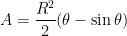
$A = \displaystyle \frac{R^2}{2} (\theta - \sin \theta)$

The thought occurred to me that $\theta$ was the first term in the Taylor series expansion of $\sin \theta$ about $\theta = 0$ , and perhaps there was a way to use this picture to generate the remaining terms of the Taylor series.

This insight led to a paper which was published in College Mathematics Journal: cmj38-1-058-059. To my surprise and delight, this paper was later selected for inclusion in The Calculus Collection: A Resource for AP and Beyond, which is a collection of articles from the publications of Mathematical Association of America specifically targeted toward teachers of AP Calculus.

Although not included in the article, it can be proven that this iterative method does indeed yield the successive Taylor polynomials of $\sin \theta$ , adding one extra term with each successive step.

I carefully scaffolded these steps into a project that I twice assigned to my TAMS precalculus students. Both semesters, my students got it… and they were impressed to know the formula that their calculators use to compute $\sin \theta$ . So I think this project is entirely within the grasp of precocious precalculus students.

I personally don’t know of a straightforward way of obtaining the expansion of $\cos \theta$ without calculus. However, once the expansion of $\sin \theta$ is known, the expansion of $\cos \theta$ can be surmised without calculus. To do this, we note that

$\cos \theta = 1 - 2 \sin^2 \left( \displaystyle \frac{\theta}{2} \right) = 1 - 2 \left( \displaystyle \frac{\theta}{2} - \frac{(\theta/2)^3}{3!} + \frac{(\theta/2)^5}{5!} \dots \right)^2$

Truncating the series after $n$ terms and squaring — and being very careful with the necessary simplifications — yield the first $n$ terms in the Taylor series of $\cos \theta$ .

Arctangents and showmanship

This story comes from Fall 1996, my first semester as a college professor. I was teaching a Precalculus class, and the topic was vectors. I forget the exact problem (believe me, I wish I could remember it), but I was going over the solution of a problem that required finding $\tan^{-1}(7)$ . I told the class that I had worked this out ahead of time, and that the approximate answer was $82^o$ . Then I used that angle for whatever I needed it for and continued until obtaining the eventual solution.

(By the way, I now realize that I was hardly following best practices by computing that angle ahead of time. Knowing what I know now, I should have brought a calculator to class and computed it on the spot. But, as a young professor, I was primarily concerned with getting the answer right, and I was petrified of making a mistake that my students could repeat.)

After solving the problem, I paused to ask for questions. One student asked a good question, and then another.

Then a third student asked, “How did you know that $\tan^{-1}(7)$ was $82^o$ ?

Suppressing a smile, I answered, “Easy; I had that one memorized.”

The class immediately erupted… some with laughter, some with disbelief. (I had a terrific rapport with those students that semester; part of the daily atmosphere was the give-and-take with any number of exuberant students.) One guy in the front row immediately challenged me: “Oh yeah? Then what’s $\tan^{-1}(9)$ ?

I started to stammer, “Uh, um…”

“Aha!” they said. “He’s faking it.” They start pulling out their calculators.

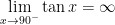
Then I thought as fast as I could. Then I realized that I knew that $\tan 82^o \approx 7$ , thanks to my calculation prior to class. I also knew that $\displaystyle \lim_{x \to 90^-} \tan x = \infty$ since the graph of $y = \tan x$ has a vertical asymptote at $x = \pi/2 = 90^o$ . So the solution to $\tan x = 9$ had to be somewhere between $82^o$ and $90^o$ .

So I took a total guess. “ $84^o$ ,” I said, faking complete and utter confidence.

Wouldn’t you know it, I was right. (The answer is about $83.66^o$ .)

In stunned disbelief, the guy who asked the question asked, “How did you do that?”

I was reeling in shock that I guessed correctly. But I put on my best poker face and answered, “I told you, I had it memorized.” And then I continued with the next example. For the rest of the semester, my students really thought I had it memorized.

To this day, this is my favorite stunt that I ever pulled off in front of my students.

Why does 0! = 1? (Part 2)

This common question arises because $0!$ does not fit the usual definition for $n!$ . Recall that, for positive integers, we have

$5! = 5 \cdot 4 \cdot 3 \cdot 2 \cdot 1 = 120$

$4! = 4 \cdot 3 \cdot 2 \cdot 1 = 24$

$3! = 3 \cdot 2 \cdot 1 = 6$

$2! = 2 \cdot 1 = 2$

$1! = 1$

In Part 1 of this series, I discussed descending down this lines with repeated division to define $0!$ .

Here’s a second way of explaining why $0!=1$ that may or may not be as convincing as the first explanation. Let’s count the number of “words” that can made using each of the three letters A, B, and C exactly once. Ignoring that most of these don’t appear in the dictionary, there are six possible words:

ABC, ACB, BAC, BCA, CAB, CBA

With two letters, there are only two possible words: AB and BA.

With four letters, there are 24 possible words:

ABCD, ABDC, ACBD, ACDB, ADBC, ADCB,
BACD, BADC, BCAD, BCDA, BDAC, BDCA,
CABD, CADB, CBAD, CBDA, CDAB, CDBA,
DABC, DACB, DBAC, DBCA, DCAB, DCBA.

Evidently, there are $4!$ different words using four letters, $3!$ different words using three letters, and $2!$ different words using two letters.

Why does this happen? Let’s examine the case of four letters. First, there are $4$ different possible choices for the first letter in the word. Next, the second letter can be anything but the first letter, so there are $3$ different possibilities for the second letter. Then there are $2$ remaining possibilities for the third letter, leaving $1$ possibility for the last.

In summary, there are $4 \cdot 3 \cdot 2 \cdot 1$ , or $4!$ , different possible words. The same logic applies for words formed from three letters or any other number of letters.

What if there are 0 letters? Then there is only 1 possibility: not making any words. So it’s reasonable to define $0!=1$ .

green line

It turns out that there’s a natural way to define $x!$ for all complex numbers $x$ that are not negative integers. For example, there’s a reasonable way to define $\left( \frac{1}{2} \right)!$ , $\left(- \frac{7}{3} \right)!$ and even $(1+2i)!$ . I’ll probably discuss this in a future post.

Why does 0! = 1? (Part 1)

This common question arises because $0!$ does not fit the usual definition for $n!$ . Recall that, for positive integers, we have

$5! = 5 \cdot 4 \cdot 3 \cdot 2 \cdot 1 = 120$

$4! = 4 \cdot 3 \cdot 2 \cdot 1 = 24$

$3! = 3 \cdot 2 \cdot 1 = 6$

$2! = 2 \cdot 1 = 2$

$1! = 1$

Going from the bottom line to the top, we see that start at $1$ , and then multiply by $2$ , then multiply by $3$ , then multiply by $4$ , then multiply by $5$ . To get $6!$ , we multiply the top line by $6$ :

$6! = 6 \cdot 5! = 6 \cdot 120 = 720$ .

Because they’re formed by successive multiplications, the factorials get large very, very quickly. I still remember, years ago, writing lesson plans while listening to the game show Wheel of Fortune. After the contestant solved the final puzzle, Pat Sajak happily announced, “You’ve just won $40,320 in cash and prizes.” My instantaneous reaction: “Ah… that’s $8!$ .” Then I planted a firm facepalm for having factorials as my first reaction. (Perhaps not surprisingly, I was still single when this happened.)

Back to $0!$ . We can also work downward as well as upward through successive division. In other words,

$5!$ divided by $5$ is equal to $4!$ .

$4!$ divided by $4$ is equal to $3!$ .

$3!$ divided by $3$ is equal to $2!$ .

$2!$ divided by $2$ is equal to $1!$ .

Clearly, there’s one more possible step: dividing by $1$ . And so we define $0!$ to be equal to $1!$ divided by $1$ , or

$0! = \displaystyle \frac{1!}{1} = 1$ .

Notice that there’s a natural way to take another step because division by 0 is not permissible. So we can define $0!$ , but we can’t define $(-1)!, (-2)!, \dots$ .

In Part 2, I’ll present a second way of approaching this question.

Engaging students: Solving exponential equations

I plan to share some of the best of these ideas on this blog (after asking my students’ permission, of course).

This student submission comes from my former student Jesse Faltys. Her topic: solving exponential equations.

APPLICATIONS: What interesting (i.e., uncontrived) word problems using this topic can your students do now?

Once your students have learned how to solve exponential equations, they can solve many different kinds of applied problems like population growth, bacterial decay, and even investment earning interest rate. (Examples Found: http://www.education.com/study-help/article/pre-calculus-help-log-expo-applications/)

Examples

1. How long will it take for $1000 to grow to $1500 if it earns 8% annual interest, compounded monthly?

$A = P \left( 1 + \displaystyle \frac{r}{n} \right)^{nt}$

$A (t) = 1500$ , $P = 1000$ , $r = 0.08$ , and $n = 12$ .
We do not know $t$ .
We will solve this equation for $t$ and will round up to the nearest month.
In five years and one month, the investment will grow to about $1500.

2. A school district estimates that its student population will grow about 5% per year for the next 15 years. How long will it take the student population to grow from the current 8000 students to 12,000?

We will solve for t in the equation $12,000 = 8000 e^{0.05t}$ .

$12,000 = 8000 e^{0.05t}$

$1.5 = e^{0.05t}$

$0.05t = \ln 1.5$

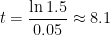
$t = \displaystyle \frac{\ln 1.5}{0.05} \approx 8.1$

The population is expected to reach 12,000 in about 8 years.

3. At 2:00 a culture contained 3000 bacteria. They are growing at the rate of 150% per hour. When will there be 5400 bacteria in the culture?

A growth rate of 150% per hour means that $r = 1.5$ and that $t$ is measured in hours.

$5400 = 3000 e^{1.5t}$

$1.8 = e^{1.5t}$

$1.5t = \ln 1.8$

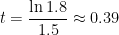
$t = \displaystyle \frac{\ln 1.8}{1.5} \approx 0.39$

At about 2:24 ( $0.39 \times 60 = 23.4$ minutes) there will be 5400 bacteria.

A note from me: this last example is used in doctor’s offices all over the country. If a patient complains of a sore throat, a swab is applied to the back of the throat to extract a few bacteria. Bacteria are of course very small and cannot be seen. The bacteria are then swabbed to a petri dish and then placed into an incubator, where the bacteria grow overnight. The next morning, there are so many bacteria on the petri dish that they can be plainly seen. Furthermore, the shapes and clusters that are formed are used to determine what type of bacteria are present.

CURRICULUM — How does this topic extend what your students should have learned in previous courses?

The students need to have a good understanding of the properties of exponents and logarithms to be able to solve exponential equations. By using properties of exponents, they should know that if both sides of the equations are powers of the same base then one could solve for x. As we all know, not all exponential equations can be expressed in terms of a common base. For these equations, properties of logarithms are used to derive a solution. The students should have a good understanding of the relationship between logarithms and exponents. Logs are the inverses of exponentials. This understanding will allow the student to be able to solve real applications by converting back and forth between the exponent and log form. That is why it is extremely important that a great review lesson is provided before jumping into solving exponential equations. The students will be in trouble if they have not successfully completed a lesson on these properties.

Technology – How can technology be used to effectively engage students with this topic?

1. Khan Academy provides a video titled “Word Problem Solving – Exponential Growth and Decay” which shows an example of a radioactive substance decay rate. The instructor on the video goes through how to organize the information from the world problem, evaluate in a table, and then solve an exponential equation. For our listening learners, this reiterates to the student the steps in how to solve exponential equations.

(http://www.khanacademy.org/math/trigonometry/exponential_and_logarithmic_func/exp_growth_decay/v/exponential-growth-functions)

2. Math warehouse is an amazing website that allows the students to interact by providing probing questions to make sure they are on the right train of thought.

For example, the question is $9^x = 27^2$ and the student must solve for $x$ . The first “hint” the website provides is “look at the bases. Rewrite them as a common base” and then the website shows them the work. The student will continue hitting the “next” button until all steps are complete. This is allowing the visual learners to see how to write out each step to successfully complete the problem.

(http://www.mathwarehouse.com/algebra/exponents/solve-exponential-equations-how-to.php)

Laws of Logarithms

One of the most common student mistakes with logarithms is thinking that

$\log_b(x+y) = \log_b x + \log_b y$ .

When I first started my career, I referred to this as the Third Classic Blunder. The first classic blunder, of course, is getting into a major land war in Asia. The second classic blunder is getting into a battle of wits with a Sicilian when death is on the line. And the third classic blunder is thinking that $\log_b(x+y)$ somehow simplfies as $\log_b x + \log_b y$ .

Sadly, as the years pass, fewer and fewer students immediately get the cultural reference. On the bright side, it’s also an opportunity to introduce a new generation to one of the great cinematic masterpieces of all time.

One of my colleagues calls this mistake the Universal Distributive Law, where the $\log_b$ distributes just as if $x+y$ was being multiplied by a constant. Other mistakes in this vein include $\sqrt{x+y} = \sqrt{x} + \sqrt{y}$ and $(x+y)^2 = x^2 + y^2$ .

Along the same lines, other classic blunders are thinking that

$\left(\log_b x\right)^n$ simplifies as $\log_b \left(x^n \right)$

and that

$\displaystyle \frac{\log_b x}{\log_b y}$ simplifies as $\log_b \left( \frac{x}{y} \right)$ .

I’m continually amazed at the number of good students who intellectually know that the above equations are false but panic and use them when solving a problem.