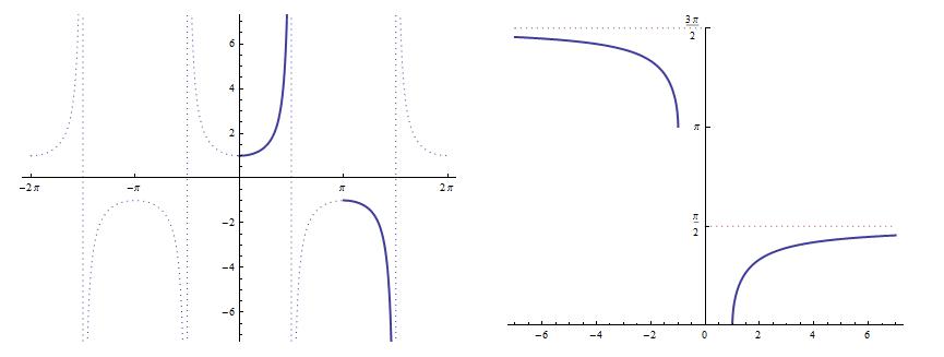
We now turn to a little-taught and perhaps controversial inverse function: arcsecant. As we’ve seen throughout this series, the domain of this inverse function must be chosen so that the graph of  satisfies the horizontal line test. It turns out that the choice of domain has surprising consequences that are almost unforeseeable using only the tools of Precalculus.
The standard definition of  uses the interval
 ![[0,\pi]](https://s0.wp.com/latex.php?latex=%5B0%2C%5Cpi%5D&bg=ffffff&fg=000000&s=0&c=20201002) — or, more precisely,
— or, more precisely, ![[0,\pi/2) \cup (\pi/2, \pi]](https://s0.wp.com/latex.php?latex=%5B0%2C%5Cpi%2F2%29+%5Ccup+%28%5Cpi%2F2%2C+%5Cpi%5D&bg=ffffff&fg=000000&s=0&c=20201002) to avoid the vertical asymptote at
to avoid the vertical asymptote at  — in order to approximately match the range of
  . However, when I was a student, I distinctly remember that my textbook chose
 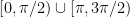 as the range for
  .
.
I believe that this definition has fallen out of favor today. However, for the purpose of today’s post, let’s just run with this definition and see what happens. This portion of the graph of is perhaps unorthodox, but it satisfies the horizontal line test so that the inverse function can be defined.

Let’s fast-forward a couple of semesters and use implicit differentiation (see also https://meangreenmath.com/2014/08/08/different-definitions-of-logarithm-part-8/ for how this same logic is used for other inverse functions) to find the derivative of :


At this point, the object is to convert the left-hand side to something involving only  . Clearly, we can replace
  with . As it turns out, the replacement of
  is a lot simpler than we saw in yesterday’s post. Once again, we begin with one of the Pythagorean identities:
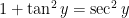


So which is it, the positive answer or the negative answer? In yesterday’s post, the answer depended on whether was positive or negative. However, with the current definition of , we know for certain that the answer is the positive one! How can we be certain? The angle  must lie in either the interval
  or else the interval
  . In either interval, is positive. So, using this definition of , we can simply say that
 ,
,
and we don’t have to worry about  that appeared in yesterday’s post.

 Turning to integration, we now have the simple formula

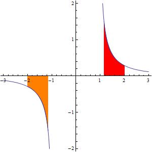
that works whether is positive or negative. For example, the orange area can now be calculated correctly:


So, unlike yesterday’s post, this definition of produces a simple integration formula.
So why isn’t this the standard definition for ? I’m afraid the answer is simple: with this definition, the equation

is no longer correct if  . Indeed, I distinctly remember thinking, back when I was a student taking trigonometry, that the definition of seemed really odd, and it seemed to me that it would be better if it matched that of . Of course, at that time in my mathematical development, it would have been almost hopeless to explain that the range had been chosen to simplify certain integrals from calculus.
So I suppose that The Powers That Be have decided that it’s more important for this identity to hold than to have a simple integration formula for 
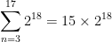
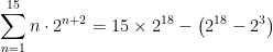
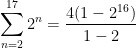
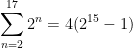
 Part 1: Introduction and statement of problem
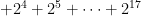
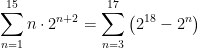
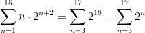
 and
and  , the number of 2-tiles and 4-tiles (respectively) that appeared throughout the course of the game:
 .
.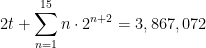


 terms, common ratio of 2, and initial term
  . Therefore,
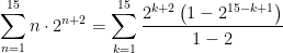


 . So
. So

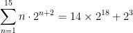

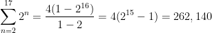


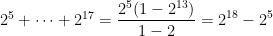

 .
.

 ,
,

 satisfies the horizontal line test for any
  or
or  . For example,
 ,
, is
is
 and
and  , with
  in the appropriate quadrant. This is analogous to converting from rectangular coordinates to polar coordinates.
 in the case that
  is a complex number.
 be a complex number so that
  . Then we define
 .
. . However, this complex logarithm doesn’t always work the way you’d think it work. For example,
 .
.
 .
.![\log \left[ (-1) \cdot (-1) \right] = \log 1 = 0](https://s0.wp.com/latex.php?latex=%5Clog+%5Cleft%5B+%28-1%29+%5Ccdot+%28-1%29+%5Cright%5D+%3D+%5Clog+1+%3D+0&bg=ffffff&fg=000000&s=0&c=20201002) ,
, .
.


 is both positive and negative on the interval
 . With this substitution:
 , and
, and


 with
with  .
. 
 is negative on the interval
 ![[2\pi/3,\pi]](https://s0.wp.com/latex.php?latex=%5B2%5Cpi%2F3%2C%5Cpi%5D&bg=ffffff&fg=000000&s=0&c=20201002) . Therefore, for this problem, we should replace
. Therefore, for this problem, we should replace  .
.


![= \displaystyle \bigg[ 3 \theta - 3 \tan \theta \bigg]_{2\pi/3}^{\pi}](https://s0.wp.com/latex.php?latex=%3D+%5Cdisplaystyle+%5Cbigg%5B+3+%5Ctheta+-+3+%5Ctan+%5Ctheta+%5Cbigg%5D_%7B2%5Cpi%2F3%7D%5E%7B%5Cpi%7D&bg=ffffff&fg=000000&s=0&c=20201002)
![= \displaystyle \left[ 3 \pi - 3 \tan \pi \right] - \left[ 3 \left( \frac{2\pi}{3} \right) - 3 \tan \left( \frac{2\pi}{3} \right) \right]](https://s0.wp.com/latex.php?latex=%3D+%5Cdisplaystyle+%5Cleft%5B+3+%5Cpi+-+3+%5Ctan+%5Cpi+%5Cright%5D+-+%5Cleft%5B+3+%5Cleft%28+%5Cfrac%7B2%5Cpi%7D%7B3%7D+%5Cright%29+-+3+%5Ctan+%5Cleft%28+%5Cfrac%7B2%5Cpi%7D%7B3%7D+%5Cright%29+%5Cright%5D&bg=ffffff&fg=000000&s=0&c=20201002)


 .
. (so that
  ), then
  .
. (so that
  ), then
  .
.


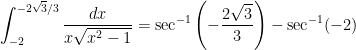
 , so that
 ![[2\sqrt{3}/3,2]](https://s0.wp.com/latex.php?latex=%5B2%5Csqrt%7B3%7D%2F3%2C2%5D&bg=ffffff&fg=000000&s=0&c=20201002) may be correctly computed as
may be correctly computed as


![[-2,-2\sqrt{3}/3]](https://s0.wp.com/latex.php?latex=%5B-2%2C-2%5Csqrt%7B3%7D%2F3%5D&bg=ffffff&fg=000000&s=0&c=20201002) is incorrectly computed using this formula!
is incorrectly computed using this formula!


 . This is perhaps not surprising since, when both are defined,
  and
and  are reciprocals.
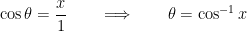 .
. .
. — that is, for
  and
and  .
. and
and  can be found using the formula
 .
. and
and  axis.
axis.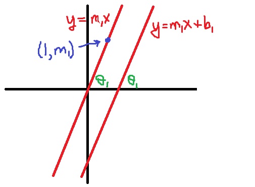
 is entirely superfluous to finding the angle
  . The important thing that matters is the slope of the line, not where the line intersects the
  axis.
axis. lies on the line
  can be found by dividing the
  .
.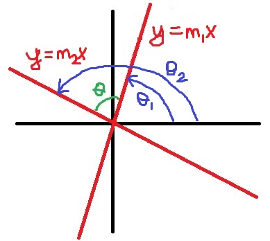
 .
. or
or  , depending on the values of
  and
and  . Let’s now compute both
  and
and  using the formula for the difference of two angles:

 and
and  , the value of
  … for now, we’ll ignore this special case). Therefore, whichever of the above two lines holds, it must be that
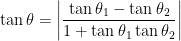
 and
and  :
:

 , and the right hand side is also undefined if
  . This matches the theorem that the two lines are perpendicular if and only if
  , or that the slopes of the two lines are negative reciprocals.