In this series of posts, I’d like to describe what I tell my students on the very first day of Calculus I. On this first day, I try to set the table for the topics that will be discussed throughout the semester. I should emphasize that I don’t hold students immediately responsible for the content of this lecture. Instead, this introduction, which usually takes 30-45 minutes, depending on the questions I get, is meant to help my students see the forest for all of the trees. For example, when we start discussing somewhat dry topics like the definition of a continuous function and the Mean Value Theorem, I can always refer back to this initial lecture for why these concepts are ultimately important.
I begin by noting the different topics that appear in Precalculus, which they should have taken in the recent past:
The definition of a function and an inverse function
Graphing polynomials and rational functions
Properties and applications of exponential and logarithmic functions
Trigonometry
Sequences and series
These different topics, when taught in Precalculus, really don’t talk to one another. With a couple of exceptions, it feels like five different units being squeezed into the same course. I’ll present a visual image of laying down an imaginary brick on the floor, and then laying down a second brick next to the first one, and so on. The above topics (with a couple of exceptions) really don’t build upon each other; they’re lateral to one another. In other words, these topics made the foundation necessary for the study of calculus. After all, the class was called Pre-Calculus.
Now that we’re in calculus, I tell my students, we’re going to have topics that build on this foundation, and the topics will build on each other. Continuing the building image, I’ll start laying imaginary bricks on the initial foundation, building vertically higher and higher, noting that the topics that we’ll see in Weeks 13 and 14 will ultimately be built upon the topics that we’ll talk about in Weeks 1 and 2. Unlike Precalculus, the topics in Calculus are explicitly interconnected, building up a body of thought from the foundation of Precalculus.
So the good news is that, unlike Precalculus, Calculus I will be an incrementally developed course from start to finish. The bad news, of course, is that Calculus I will be an incrementally developed course from start to finish. In Precalculus, if you didn’t particularly like one topic (say, logarithms), that really would not affect your success later on with a future topic (say, trigonometry). However, in Calculus, the whole course is put together from start to finish.
The good news is that while there are many interconnected topics in calculus, there are going to be two themes that run throughout the course:
Approximating curved things by straight things, and
Passing to limits
And we’re going to be applying these two themes again and again throughout the semester. (I wish I could take credit for synthesizing the topics of calculus into these two themes, but I learned this idea from my own calculus professor back in the mid-1980s.)
For the remainder of this first lecture, I show how these two themes apply to two completely different problems:
Finding the speed of a falling object when it hits the ground.
Finding the area under the curve between and .
I’ll describe how I present these to new calculus students in the coming posts.
Math majors are completely comfortable with the formula for the area of a circle. However, they often tell me that they don’t remember a proof or justification for why this formula is true. And they certainly don’t remember a justification that would be appropriate for showing geometry students.
In this series of posts, I’ll discuss several ways that the area of a circle can be found using calculus. I’ll also discuss a straightforward classroom activity by which students can discover for themselves why .If denotes a circular region with radius centered at the origin, then
This double integral may be computed by converting to polar coordinates. The distance from the origin varies from to , while the angle varies from to . Using the conversion, we see that
We note that the above proof uses the fact that calculus with trigonometric functions must be done with radians and not degrees. In other words, we had to change the range of integration to and not .
Math majors are completely comfortable with the formula for the area of a circle. However, they often tell me that they don’t remember a proof or justification for why this formula is true. And they certainly don’t remember a justification that would be appropriate for showing geometry students.
In this series of posts, I’ll discuss several ways that the area of a circle can be found using calculus. I’ll also discuss a straightforward classroom activity by which students can discover for themselves why .
A circle centered at the origin with radius may be viewed as the region between and . These two functions intersect at and . Therefore, the area of the circle is the integral of the difference of the two functions:
This may be evaluated by using the trigonometric substitution and changing the range of integration to to . Since , we find
We note that the above proof uses the fact that calculus with trigonometric functions must be done with radians and not degrees. In other words, we had to change the range of integration to and not .
Math majors are completely comfortable with the formula for the area of a circle. However, they often tell me that they don’t remember a proof or justification for why this formula is true. And they certainly don’t remember a justification that would be appropriate for showing geometry students.
In this series of posts, I’ll discuss several ways that the area of a circle can be found using calculus. I’ll also discuss a straightforward classroom activity by which students can discover for themselves why .In the first few weeks after a calculus class, after students are introduced to the concept of limits, the derivative is introduced for the first time… often as the slope of a tangent line to the curve. Here it is: if $y = f(x)$, then
From this definition, the first few rules of differentiation are derived in approximately the following order:
1. If , a constant, then .
2. If and are both differentiable, then .
3. If is differentiable and is a constant, then .
4. If , where is a nonnegative integer, then . This may be proved by at least two different techniques:
The binomial expansion
The Product Rule (derived later) and mathematical induction
5. If is a polynomial, then . In other words, taking the derivative of a polynomial is easy.
After doing a few examples to help these concepts sink in, I’ll show the following two examples with about 3-4 minutes left in class.
Example 1. Let . Notice I’ve changed the variable from to , but that’s OK. Does this remind you of anything? (Students answer: the area of a circle.) What’s the derivative? Remember, is just a constant. So . Does this remind you of anything? (Students answer: Whoa… the circumference of a circle.)
Example 2. Now let’s try . Does this remind you of anything? (Students answer: the volume of a sphere.) What’s the derivative? Again, is just a constant. So . Does this remind you of anything? (Students answer: Whoa… the surface area of a sphere.)
Hmmm. That’s interesting. The derivative of the area of a circle is the circumference of the circle, and the derivative of the area of a sphere is the surface area of the sphere. I wonder why this works. Any ideas? (Students: stunned silence.)
This is what’s known on television as a cliff-hanger, and I’ll give you the answer at the start of class tomorrow. (Students groan, as they really want to know the answer immediately.)
In the spirit of a cliff-hanger, I offer the following thought bubble before presenting the answer.
By definition, if , then
The numerator may be viewed as the area of the ring between concentric circles with radii and . In other words, imagine starting with a solid red disk of radius and then removing a solid white disk of radius . The picture would look something like this:
Notice that the ring has a thickness of . If this ring were to be “unpeeled” and flattened, it would approximately resemble a rectangle. The height of the rectangle would be , while the length of the rectangle would be the circumference of the circle. So
and we can conclude that
By the same reasoning, the derivative of the volume of a sphere ought to be the surface area of the sphere.
Pedagogically, I find that the above discussion helps reinforce the definition of a derivative at a time when students are most willing to forget about the formal definition in favor of the various rules of differentiation.
In the above work, we started with the formula for the area of the circle and then confirmed that its derivative matched the expected result. However, the above logic can be used to derive the formula for the area of a circle from the formula $C(r) = 2\pi r$ for the circumference. We begin with the observation that , as above. Therefore, by the Fundamental Theorem of Calculus,
Since the area of a circle with radius is , we conclude that .
Pedagogically, I don’t particularly recommend this approach, as I think students would find this explanation more confusing than the first approach. However, I can see that this could be useful for reinforcing the statement of the Fundamental Theorem of Calculus.
By the way, the above reasoning works for a square or cube also, but with a little twist. For a square of side length , the area is and the perimeter is , which isn’t the derivative of . The reason this didn’t work is because the side length of a square corresponds to the diameter of a circle, not the radius of a circle.
But, if we let denote half the side length of a square, then the above logic works out since
and
Written in terms of the half-sidelength , we see that .
Throughout grades K-10, students are slowly introduced to the concept of angles. They are told that there are degrees in a right angle, degrees in a straight angle, and a circle has degrees. They are introduced to and right triangles. Fans of snowboarding even know the multiples of degrees up to or even degrees.
Then, in Precalculus, we make students get comfortable with , , , , , and multiples thereof.
We tell students that radians and degrees are just two ways of measuring angles, just like inches and centimeters are two ways of measuring the length of a line segment.
Still, students are extremely comfortable with measuring angles in degrees. They can easily visualize an angle of , but to visualize an angle of radians, they inevitably need to convert to degrees first. In his book Surely You’re Joking, Mr. Feynman!, Nobel-Prize laureate Richard P. Feynman described himself as a boy:
I was never any good in sports. I was always terrified if a tennis ball would come over the fence and land near me, because I never could get it over the fence – it usually went about a radian off of where it was supposed to go.
Naturally, students wonder why we make them get comfortable with measuring angles with radians.
The short answer, appropriate for Precalculus students: Certain formulas are a little easier to write with radians as opposed to degrees, which in turn make certain formulas in calculus a lot easier.
The longer answer, which Precalculus students would not appreciate, is that radian measure is needed to make the derivatives of and look palatable.
In both of these formulas, the angle must be measured in radians.
Students may complain that it’d be easy to make a formula of is measured in degrees, and they’d be right:
and
However, getting rid of the makes the following computations from calculus a lot easier.
2a. Early in calculus, the limit
is derived using the Sandwich Theorem (or Pinching Theorem or Squeeze Theorem). I won’t reinvent the wheel by writing out the proof, but it can be found here. The first step of the proof uses the formula for the above formula for the area of a circular sector.
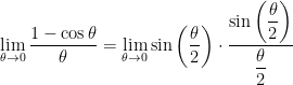
2b. Using the trigonometric identity , we replace by to find
3. Both of the above limits — as well as the formulas for and — are needed to prove that and . Again, I won’t reinvent the wheel, but the proofs can be found here.
So, to make a long story short, radians are used to make the derivatives $y = \sin x$ and $y = \cos x$ easier to remember. It is logically possible to differentiate these functions using degrees instead of radians — see http://www.math.ubc.ca/~feldman/m100/sinUnits.pdf. However, possible is not the same thing as preferable, as calculus is a whole lot easier without these extra factors of floating around.
So as the base gets closer to , the answer remains . So, from this perspective, it looks like ought to be equal to .
In conclusion: looking at it one way, should be defined to be . From another perspective, should be defined to be .
Of course, we can’t define a number to be two different things! So we’ll just say that is undefined — just like dividing by is undefined — rather than pretend that switches between two different values.
Here’s a more technical explanation about why is an indeterminate form, using calculus.
Part 1. As before,
.
The first equality is true because, inside of the limit, is permitted to get close to but cannot actually equal , and there’s no ambiguity about if . (Naturally, is undefined if .)
The second equality is true because the limit of a constant is the constant.
Part 2. As before,
.
Once again, the first equality is true because, inside of the limit, is permitted to get close to but cannot actually equal , and there’s no ambiguity about if .
As before, the answers from Parts 1 and 2 are different. But wait, there’s more…
Part 3. Here’s another way that can be considered, just to give us a headache. Let’s evaluate
Clearly, the base tends to as . Also, as , so that as . In other words, this limit has the indeterminate form .
To evaluate this limit, let’s take a logarithm under the limit:
Therefore, without the extra logarithm,
Part 4. It gets even better. Let be any positive real number. By the same logic as above,
So, for any , we can find a function of the indeterminate form so that .
In other words, we could justify defining to be any nonnegative number. Clearly, it’s better instead to simply say that is undefined.
P.S. I don’t know if it’s possible to have an indeterminate form of where the answer is either negative or infinite. I tend to doubt it, but I’m not sure.
Here’s a simple probability problem that should be accessible to high school students who have learned the Multiplication Rule:
Suppose that you play the lottery every day for about 20 years. Each time you play, the chance that you win is chance in . What is the probability that, after playing times, you never win?
This is a straightforward application of the Multiplication Rule from probability. The chance of not winning on any one play is . Therefore, the chance of not winning consecutive times is , which we can approximate with a calculator.
Well, that was easy enough. Now, just for the fun of it, let’s find the reciprocal of this answer.
Hmmm. Two point seven one. Where have I seen that before? Hmmm… Nah, it couldn’t be that.
What if we changed the number in the above problem to ? Then the probability would be .
There’s no denying it now… it looks like the reciprocal is approximately , so that the probability of never winning for both problems is approximately .
Why is this happening? I offer a thought bubble if you’d like to think about this before proceeding to the answer.
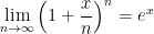
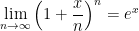
The above calculations are numerical examples that demonstrate the limit
In particular, for the special case when , we find
The first limit can be proved using L’Hopital’s Rule. By continuity of the function , we have
The right-hand side has the form as , and so we may use L’Hopital’s rule, differentiating both the numerator and the denominator with respect to .
Applying the exponential function to both sides, we conclude that
The above calculation also justifies (in Algebra II and Precalculus) how the formula for continuous compound interest can be derived from the formula for discrete compound interest
All this to say, Euler knew what he was doing when he decided that was so important that it deserved to be named.
This is the last in a series of posts about square roots and other roots, hopefully providing a deeper look at an apparently simple concept. However, in this post, we discuss how calculators are programmed to compute square roots quickly.
Today’s movie clip, therefore, is set in modern times:
So how do calculators find square roots anyway? First, we recognize that is a root of the polynomial . Therefore, Newton’s method (or the Newton-Raphson method) can be used to find the root of this function. Newton’s method dictates that we begin with an initial guess and then iteratively find the next guesses using the recursively defined sequence
For the case at hand, since , we may write
,
which reduces to
This algorithm can be programmed using C++, Python, etc.. For pedagogical purposes, however, I’ve found that a spreadsheet like Microsoft Excel is a good way to sell this to students. In the spreadsheet below, I use Excel to find . In cell A1, I entered as a first guess for . Notice that this is a really lousy first guess! Then, in cell A2, I typed the formula
=1/2*(A1+2000/A1)
So Excel computes
.
Then I filled down that formula into cells A3 through A16.
Notice that this algorithm quickly converges to , even though the initial guess was terrible. After 7 steps, the answer is only correct to 2 significant digits (). After 8 steps, the answer is correct to 4 significant digits (). On the 9th step, the answer is correct to 9 significant digits ().
Indeed, there’s a theorem that essentially states that, when this algorithm converges, the number of correct digits basically doubles with each successive step. That’s a lot better than the methods shown at the start of this series of posts which only produced one extra digit with each step.
This algorithm works for finding th roots as well as square roots. Since is a root of , Newton’s method reduces to
,
which reduces to the above sequence if .
See also this Wikipedia page for further historical information as well as discussion about how the above recursive sequence can be obtained without calculus.
This is the fifth in a series of posts about calculating roots without a calculator, with special consideration to how these tales can engage students more deeply with the secondary mathematics curriculum. As most students today have a hard time believing that square roots can be computed without a calculator, hopefully giving them some appreciation for their elders.
Today’s story takes us back to a time before the advent of cheap pocket calculators: 1949.
The following story comes from the chapter “Lucky Numbers” of Surely You’re Joking, Mr. Feynman!, a collection of tales by the late Nobel Prize winning physicist, Richard P. Feynman. Feynman was arguably the greatest American-born physicist — the subject of the excellent biography Genius: The Life and Science of Richard Feynman — and he had a tendency to one-up anyone who tried to one-up him. (He was also a serial philanderer, but that’s another story.) Here’s a story involving how, in the summer of 1949, he calculated without a calculator.
The first time I was in Brazil I was eating a noon meal at I don’t know what time — I was always in the restaurants at the wrong time — and I was the only customer in the place. I was eating rice with steak (which I loved), and there were about four waiters standing around.
A Japanese man came into the restaurant. I had seen him before, wandering around; he was trying to sell abacuses. (Note: At the time of this story, before the advent of pocket calculators, the abacus was arguably the world’s most powerful hand-held computational device.) He started to talk to the waiters, and challenged them: He said he could add numbers faster than any of them could do.
The waiters didn’t want to lose face, so they said, “Yeah, yeah. Why don’t you go over and challenge the customer over there?”
The man came over. I protested, “But I don’t speak Portuguese well!”
The waiters laughed. “The numbers are easy,” they said.
They brought me a paper and pencil.
The man asked a waiter to call out some numbers to add. He beat me hollow, because while I was writing the numbers down, he was already adding them as he went along.
I suggested that the waiter write down two identical lists of numbers and hand them to us at the same time. It didn’t make much difference. He still beat me by quite a bit.
However, the man got a little bit excited: he wanted to prove himself some more. “Multiplição!” he said.
Somebody wrote down a problem. He beat me again, but not by much, because I’m pretty good at products.
The man then made a mistake: he proposed we go on to division. What he didn’t realize was, the harder the problem, the better chance I had.
We both did a long division problem. It was a tie.
This bothered the hell out of the Japanese man, because he was apparently well trained on the abacus, and here he was almost beaten by this customer in a restaurant.
“Raios cubicos!” he says with a vengeance. Cube roots! He wants to do cube roots by arithmetic. It’s hard to find a more difficult fundamental problem in arithmetic. It must have been his topnotch exercise in abacus-land.
He writes down a number on some paper— any old number— and I still remember it: . He starts working on it, mumbling and grumbling: “Mmmmmmagmmmmbrrr”— he’s working like a demon! He’s poring away, doing this cube root.
Meanwhile I’m just sitting there.
One of the waiters says, “What are you doing?”.
I point to my head. “Thinking!” I say. I write down on the paper. After a little while I’ve got .
The man with the abacus wipes the sweat off his forehead: “Twelve!” he says.
“Oh, no!” I say. “More digits! More digits!” I know that in taking a cube root by arithmetic, each new digit is even more work that the one before. It’s a hard job.
He buries himself again, grunting “Rrrrgrrrrmmmmmm …,” while I add on two more digits. He finally lifts his head to say, “!”
The waiter are all excited and happy. They tell the man, “Look! He does it only by thinking, and you need an abacus! He’s got more digits!”
He was completely washed out, and left, humiliated. The waiters congratulated each other.
How did the customer beat the abacus?
The number was . I happened to know that a cubic foot contains cubic inches, so the answer is a tiny bit more than . The excess, , is only one part in nearly , and I had learned in calculus that for small fractions, the cube root’s excess is one-third of the number’s excess. So all I had to do is find the fraction , and multiply by (divide by and multiply by ). So I was able to pull out a whole lot of digits that way.
A few weeks later, the man came into the cocktail lounge of the hotel I was staying at. He recognized me and came over. “Tell me,” he said, “how were you able to do that cube-root problem so fast?”
I started to explain that it was an approximate method, and had to do with the percentage of error. “Suppose you had given me . Now the cube root of is …”
He picks up his abacus: zzzzzzzzzzzzzzz— “Oh yes,” he says.
I realized something: he doesn’t know numbers. With the abacus, you don’t have to memorize a lot of arithmetic combinations; all you have to do is to learn to push the little beads up and down. You don’t have to memorize 9+7=16; you just know that when you add 9, you push a ten’s bead up and pull a one’s bead down. So we’re slower at basic arithmetic, but we know numbers.
Furthermore, the whole idea of an approximate method was beyond him, even though a cubic root often cannot be computed exactly by any method. So I never could teach him how I did cube roots or explain how lucky I was that he happened to choose .
The key part of the story, “for small fractions, the cube root’s excess is one-third of the number’s excess,” deserves some elaboration, especially since this computational trick isn’t often taught in those terms anymore. If , then , so that . Since , the equation of the tangent line to at is
.
The key observation is that, for , the graph of will be very close indeed to the graph of . In Calculus I, this is sometimes called the linearization of at . In Calculus II, we observe that these are the first two terms in the Taylor series expansion of about .
For Feynman’s problem, , so that if $x \approx 0$. Then $\latex \sqrt[3]{1729.03}$ can be rewritten as
This last equation explains the line “all I had to do is find the fraction , and multiply by .” With enough patience, the first few digits of the correction can be mentally computed since
So Feynman could determine quickly that the answer was .
By the way,
So the linearization provides an estimate accurate to eight significant digits. Additional digits could be obtained by using the next term in the Taylor series.
I have a similar story to tell. Back in 1996 or 1997, when I first moved to Texas and was making new friends, I quickly discovered that one way to get odd facial expressions out of strangers was by mentioning that I was a math professor. Occasionally, however, someone would test me to see if I really was a math professor. One guy (who is now a good friend; later, we played in the infield together on our church-league softball team) asked me to figure out without a calculator — before someone could walk to the next room and return with the calculator. After two seconds of panic, I realized that I was really lucky that he happened to pick a number close to . Using the same logic as above,
.
Knowing that this came from a linearization and that the tangent line to lies above the curve, I knew that this estimate was too high. But I didn’t have time to work out a correction (besides, I couldn’t remember the full Taylor series off the top of my head), so I answered/guessed , hoping that I did the arithmetic correctly. You can imagine the amazement when someone punched into the calculator to get
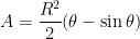
Is calculus really necessary for obtaining a Taylor series? Years ago, while perusing an old Schaum’s outline, I found a very curious formula for the area of a circular segment:
The thought occurred to me that was the first term in the Taylor series expansion of about , and perhaps there was a way to use this picture to generate the remaining terms of the Taylor series.
This insight led to a paper which was published in College Mathematics Journal: cmj38-1-058-059. To my surprise and delight, this paper was later selected for inclusion in The Calculus Collection: A Resource for AP and Beyond, which is a collection of articles from the publications of Mathematical Association of America specifically targeted toward teachers of AP Calculus.
Although not included in the article, it can be proven that this iterative method does indeed yield the successive Taylor polynomials of , adding one extra term with each successive step.
I carefully scaffolded these steps into a project that I twice assigned to my TAMS precalculus students. Both semesters, my students got it… and they were impressed to know the formula that their calculators use to compute . So I think this project is entirely within the grasp of precocious precalculus students.
I personally don’t know of a straightforward way of obtaining the expansion of without calculus. However, once the expansion of is known, the expansion of can be surmised without calculus. To do this, we note that
Truncating the series after terms and squaring — and being very careful with the necessary simplifications — yield the first terms in the Taylor series of .

between
and
.
 for the area of a circle. However, they often tell me that they don’t remember a proof or justification for why this formula is true. And they certainly don’t remember a justification that would be appropriate for showing geometry students.
 denotes a circular region with radius
  centered at the origin, then
 to
to  , while the angle varies from
  to
to  . Using the
  , we see that
![A = \displaystyle \int_0^{2\pi} \left[ \frac{r^2}{2} \right]_0^a \, d\theta](https://s0.wp.com/latex.php?latex=A+%3D+%5Cdisplaystyle+%5Cint_0%5E%7B2%5Cpi%7D+%5Cleft%5B+%5Cfrac%7Br%5E2%7D%7B2%7D+%5Cright%5D_0%5Ea+%5C%2C+d%5Ctheta&bg=ffffff&fg=000000&s=0&c=20201002)


![[0,2\pi]](https://s0.wp.com/latex.php?latex=%5B0%2C2%5Cpi%5D&bg=ffffff&fg=000000&s=0&c=20201002) and not
and not ![[0^o, 360^o]](https://s0.wp.com/latex.php?latex=%5B0%5Eo%2C+360%5Eo%5D&bg=ffffff&fg=000000&s=0&c=20201002) .
. may be viewed as the region between
  and
and  . These two functions intersect at
  and
and  . Therefore, the area of the circle is the integral of the difference of the two functions:
![A = \displaystyle \int_{-r}^r \left[g(x) - f(x) \right] \, dx= \displaystyle \int_{-r}^r 2 \sqrt{r^2 - x^2} \, dx](https://s0.wp.com/latex.php?latex=A+%3D+%5Cdisplaystyle+%5Cint_%7B-r%7D%5Er+%5Cleft%5Bg%28x%29+-+f%28x%29+%5Cright%5D+%5C%2C+dx%3D+%5Cdisplaystyle+%5Cint_%7B-r%7D%5Er+2+%5Csqrt%7Br%5E2+-+x%5E2%7D+%5C%2C+dx&bg=ffffff&fg=000000&s=0&c=20201002)
 and changing the range of integration to
  to
to  . Since
  , we find


![A = \displaystyle r^2 \left[ \theta + \frac{1}{2} \sin 2\theta \right]_{-\pi/2}^{\pi/2}](https://s0.wp.com/latex.php?latex=A+%3D+%5Cdisplaystyle+r%5E2+%5Cleft%5B+%5Ctheta+%2B+%5Cfrac%7B1%7D%7B2%7D+%5Csin+2%5Ctheta+%5Cright%5D_%7B-%5Cpi%2F2%7D%5E%7B%5Cpi%2F2%7D&bg=ffffff&fg=000000&s=0&c=20201002)
![A = \displaystyle r^2 \left[ \left( \displaystyle \frac{\pi}{2} + \frac{1}{2} \sin \pi \right) - \left( - \frac{\pi}{2} + \frac{1}{2} \sin (-\pi) \right) \right]](https://s0.wp.com/latex.php?latex=A+%3D+%5Cdisplaystyle+r%5E2+%5Cleft%5B+%5Cleft%28+%5Cdisplaystyle+%5Cfrac%7B%5Cpi%7D%7B2%7D+%2B+%5Cfrac%7B1%7D%7B2%7D+%5Csin+%5Cpi+%5Cright%29+-+%5Cleft%28+-+%5Cfrac%7B%5Cpi%7D%7B2%7D+%2B+%5Cfrac%7B1%7D%7B2%7D+%5Csin+%28-%5Cpi%29+%5Cright%29+%5Cright%5D&bg=ffffff&fg=000000&s=0&c=20201002)
![[-\pi/2,\pi/2]](https://s0.wp.com/latex.php?latex=%5B-%5Cpi%2F2%2C%5Cpi%2F2%5D&bg=ffffff&fg=000000&s=0&c=20201002) and not
and not ![[-90^o, 90^o]](https://s0.wp.com/latex.php?latex=%5B-90%5Eo%2C+90%5Eo%5D&bg=ffffff&fg=000000&s=0&c=20201002) .
.
 , a constant, then
  .
. and
and  are both differentiable, then
  .
. is a constant, then
  .
. , where
  is a nonnegative integer, then
  . This may be proved by at least two different techniques:
 is a polynomial, then
  . In other words, taking the derivative of a polynomial is easy.
 . Notice I’ve changed the variable from
  to
to  is just a constant. So
  . Does this remind you of anything? (Students answer: Whoa… the circumference of a circle.)
 . Does this remind you of anything? (Students answer: the volume of a sphere.) What’s the derivative? Again,
  is just a constant. So
  . Does this remind you of anything? (Students answer: Whoa… the surface area of a sphere.)

 . In other words, imagine starting with a solid red disk of radius
  and then removing a solid white disk of radius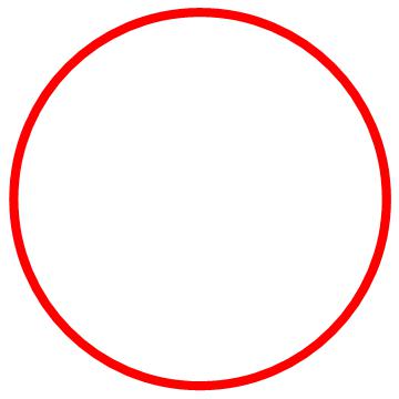
 . If this ring were to be “unpeeled” and flattened, it would approximately resemble a rectangle. The height of the rectangle would be
  , while the length of the rectangle would be the circumference of the circle. So

 , as above. Therefore, by the Fundamental Theorem of Calculus,

![A(r) - A(0) = \displaystyle \left[ \pi t^2 \right]_0^r](https://s0.wp.com/latex.php?latex=A%28r%29+-+A%280%29+%3D+%5Cdisplaystyle+%5Cleft%5B+%5Cpi+t%5E2+%5Cright%5D_0%5Er&bg=ffffff&fg=000000&s=0&c=20201002)

 is
is  , the area is
  and the perimeter is
  , which isn’t the derivative of
  . The reason this didn’t work is because the side length

 .
. degrees in a right angle,
  degrees in a straight angle, and a circle has
  degrees. They are introduced to
  and
and  right triangles. Fans of snowboarding even know the multiples of
  or even
  degrees.
 ,
,  ,
,  ,
,  , and multiples thereof.
 , but to visualize an angle of
  radians, they inevitably need to convert to degrees first. In his book
  and
and  look palatable.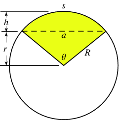
 in a circle with radius

 and
and 
 makes the following computations from calculus a lot easier.
 , we replace
  to find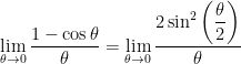


 and
and  — are needed to prove that
  and
and 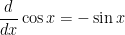 . Again, I won’t reinvent the wheel, but the proofs can be found
  floating around.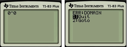
 is undefined that should be within the grasp of pre-algebra students:
 ? Of course, it’s
  ? Again,
  ? Again,
  , or
, or  ? Again,
  , or
, or ![\sqrt[3]{0}](https://s0.wp.com/latex.php?latex=%5Csqrt%5B3%5D%7B0%7D&bg=ffffff&fg=000000&s=0&c=20201002) ? In other words, what number, when cubed, is
? In other words, what number, when cubed, is  , or
, or ![\sqrt[10]{0}](https://s0.wp.com/latex.php?latex=%5Csqrt%5B10%5D%7B0%7D&bg=ffffff&fg=000000&s=0&c=20201002) ? In other words, what number, when raised to the 10th power, is
? In other words, what number, when raised to the 10th power, is  .
.  .
. . Again,
  . Again,
  ? Again,
  . Again,
  ? Again,
  .
. if
if  . (Naturally,
  is undefined if
  .)
.) .
. if
if  .
.
 . Also,
  as
as  , so that
  as
as 



 be any positive real number. By the same logic as above,
 , we can find a function
  .
. . What is the probability that, after playing
  . Therefore, the chance of not winning
  , which we can approximate with a calculator.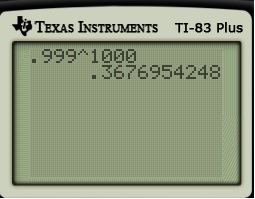

 ? Then the probability would be
  .
.
 , so that the probability of never winning for both problems is approximately
  .
.
 , we find
 , we have
![\ln \left[ \displaystyle \lim_{n \to \infty} \left(1 + \frac{x}{n}\right)^n \right] = \displaystyle \lim_{n \to \infty} \ln \left[ \left(1 + \frac{x}{n}\right)^n \right]](https://s0.wp.com/latex.php?latex=%5Cln+%5Cleft%5B+%5Cdisplaystyle+%5Clim_%7Bn+%5Cto+%5Cinfty%7D+%5Cleft%281+%2B+%5Cfrac%7Bx%7D%7Bn%7D%5Cright%29%5En+%5Cright%5D+%3D+%5Cdisplaystyle+%5Clim_%7Bn+%5Cto+%5Cinfty%7D+%5Cln+%5Cleft%5B+%5Cleft%281+%2B+%5Cfrac%7Bx%7D%7Bn%7D%5Cright%29%5En+%5Cright%5D&bg=ffffff&fg=000000&s=0&c=20201002)
![\ln \left[ \displaystyle \lim_{n \to \infty} \left(1 + \frac{x}{n}\right)^n \right] = \displaystyle \lim_{n \to \infty} n \ln \left(1 + \frac{x}{n}\right)](https://s0.wp.com/latex.php?latex=%5Cln+%5Cleft%5B+%5Cdisplaystyle+%5Clim_%7Bn+%5Cto+%5Cinfty%7D+%5Cleft%281+%2B+%5Cfrac%7Bx%7D%7Bn%7D%5Cright%29%5En+%5Cright%5D+%3D+%5Cdisplaystyle+%5Clim_%7Bn+%5Cto+%5Cinfty%7D+n+%5Cln+%5Cleft%281+%2B+%5Cfrac%7Bx%7D%7Bn%7D%5Cright%29&bg=ffffff&fg=000000&s=0&c=20201002)
![\ln \left[ \displaystyle \lim_{n \to \infty} \left(1 + \frac{x}{n}\right)^n \right] = \displaystyle \lim_{n \to \infty} \frac{ \displaystyle \ln \left(1 + \frac{x}{n}\right)}{\displaystyle \frac{1}{n}}](https://s0.wp.com/latex.php?latex=%5Cln+%5Cleft%5B+%5Cdisplaystyle+%5Clim_%7Bn+%5Cto+%5Cinfty%7D+%5Cleft%281+%2B+%5Cfrac%7Bx%7D%7Bn%7D%5Cright%29%5En+%5Cright%5D+%3D+%5Cdisplaystyle+%5Clim_%7Bn+%5Cto+%5Cinfty%7D+%5Cfrac%7B+%5Cdisplaystyle+%5Cln+%5Cleft%281+%2B+%5Cfrac%7Bx%7D%7Bn%7D%5Cright%29%7D%7B%5Cdisplaystyle+%5Cfrac%7B1%7D%7Bn%7D%7D&bg=ffffff&fg=000000&s=0&c=20201002)
 as
as  , and so we may use L’Hopital’s rule, differentiating both the numerator and the denominator with respect to
 ![\ln \left[ \displaystyle \lim_{n \to \infty} \left(1 + \frac{x}{n}\right)^n \right] = \displaystyle \lim_{n \to \infty} \frac{ \displaystyle \frac{1}{1 + \frac{x}{n}} \cdot \frac{-x}{n^2} }{\displaystyle \frac{-1}{n^2}}](https://s0.wp.com/latex.php?latex=%5Cln+%5Cleft%5B+%5Cdisplaystyle+%5Clim_%7Bn+%5Cto+%5Cinfty%7D+%5Cleft%281+%2B+%5Cfrac%7Bx%7D%7Bn%7D%5Cright%29%5En+%5Cright%5D+%3D+%5Cdisplaystyle+%5Clim_%7Bn+%5Cto+%5Cinfty%7D+%5Cfrac%7B+%5Cdisplaystyle+%5Cfrac%7B1%7D%7B1+%2B+%5Cfrac%7Bx%7D%7Bn%7D%7D+%5Ccdot+%5Cfrac%7B-x%7D%7Bn%5E2%7D+%7D%7B%5Cdisplaystyle+%5Cfrac%7B-1%7D%7Bn%5E2%7D%7D&bg=ffffff&fg=000000&s=0&c=20201002)
![\ln \left[ \displaystyle \lim_{n \to \infty} \left(1 + \frac{x}{n}\right)^n \right] = \displaystyle \lim_{n \to \infty} \displaystyle \frac{x}{1 + \frac{x}{n}}](https://s0.wp.com/latex.php?latex=%5Cln+%5Cleft%5B+%5Cdisplaystyle+%5Clim_%7Bn+%5Cto+%5Cinfty%7D+%5Cleft%281+%2B+%5Cfrac%7Bx%7D%7Bn%7D%5Cright%29%5En+%5Cright%5D+%3D+%5Cdisplaystyle+%5Clim_%7Bn+%5Cto+%5Cinfty%7D+%5Cdisplaystyle+%5Cfrac%7Bx%7D%7B1+%2B+%5Cfrac%7Bx%7D%7Bn%7D%7D&bg=ffffff&fg=000000&s=0&c=20201002)
![\ln \left[ \displaystyle \lim_{n \to \infty} \left(1 + \frac{x}{n}\right)^n \right] = \displaystyle \frac{x}{1 + 0}](https://s0.wp.com/latex.php?latex=%5Cln+%5Cleft%5B+%5Cdisplaystyle+%5Clim_%7Bn+%5Cto+%5Cinfty%7D+%5Cleft%281+%2B+%5Cfrac%7Bx%7D%7Bn%7D%5Cright%29%5En+%5Cright%5D+%3D+%5Cdisplaystyle+%5Cfrac%7Bx%7D%7B1+%2B+0%7D&bg=ffffff&fg=000000&s=0&c=20201002)
![\ln \left[ \displaystyle \lim_{n \to \infty} \left(1 + \frac{x}{n}\right)^n \right] = x](https://s0.wp.com/latex.php?latex=%5Cln+%5Cleft%5B+%5Cdisplaystyle+%5Clim_%7Bn+%5Cto+%5Cinfty%7D+%5Cleft%281+%2B+%5Cfrac%7Bx%7D%7Bn%7D%5Cright%29%5En+%5Cright%5D+%3D+x&bg=ffffff&fg=000000&s=0&c=20201002)
 can be derived from the formula for discrete compound interest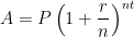
 is a root of the polynomial
  . Therefore,
  and then iteratively find the next guesses using the recursively defined sequence
 , we may write
 ,
,
 . In cell A1, I entered
  .
.
 ). After 8 steps, the answer is correct to 4 significant digits (
 ). On the 9th step, the answer is correct to 9 significant digits (
 ).
).![\sqrt[k]{a}](https://s0.wp.com/latex.php?latex=%5Csqrt%5Bk%5D%7Ba%7D&bg=ffffff&fg=000000&s=0&c=20201002) is a root of
is a root of  , Newton’s method reduces to
 ,
, .
.![\sqrt[3]{1729.03}](https://s0.wp.com/latex.php?latex=%5Csqrt%5B3%5D%7B1729.03%7D&bg=ffffff&fg=000000&s=0&c=20201002) without a calculator.
without a calculator. . He starts working on it, mumbling and grumbling: “Mmmmmmagmmmmbrrr”— he’s working like a demon! He’s poring away, doing this cube root.
 on the paper. After a little while I’ve got
  .
. !”
!” cubic inches, so the answer is a tiny bit more than
  , is only one part in nearly
  , and I had learned in calculus that for small fractions, the cube root’s excess is one-third of the number’s excess. So all I had to do is find the fraction
  , and multiply by
  (divide by
  and multiply by
  . Now the cube root of
  is
is  , then
  , so that
  . Since
  , the equation of the tangent line to
  .
. , the graph of
  will be very close indeed to the graph of
  at
at  . In Calculus II, we observe that these are the first two terms in the
  .
. , so that
 ![\sqrt[3]{1+x} \approx 1 + \frac{1}{3} x](https://s0.wp.com/latex.php?latex=%5Csqrt%5B3%5D%7B1%2Bx%7D+%5Capprox+1+%2B+%5Cfrac%7B1%7D%7B3%7D+x&bg=ffffff&fg=000000&s=0&c=20201002) if $x \approx 0$. Then $\latex \sqrt[3]{1729.03}$ can be rewritten as
if $x \approx 0$. Then $\latex \sqrt[3]{1729.03}$ can be rewritten as![\sqrt[3]{1729.03} = \sqrt[3]{1728} \sqrt[3]{ \displaystyle \frac{1729.03}{1728} }](https://s0.wp.com/latex.php?latex=%5Csqrt%5B3%5D%7B1729.03%7D+%3D+%5Csqrt%5B3%5D%7B1728%7D+%5Csqrt%5B3%5D%7B+%5Cdisplaystyle+%5Cfrac%7B1729.03%7D%7B1728%7D+%7D&bg=ffffff&fg=000000&s=0&c=20201002)
![\sqrt[3]{1729.03} = 12 \sqrt[3]{\displaystyle 1 + \frac{1.03}{1728}}](https://s0.wp.com/latex.php?latex=%5Csqrt%5B3%5D%7B1729.03%7D+%3D+12+%5Csqrt%5B3%5D%7B%5Cdisplaystyle+1+%2B+%5Cfrac%7B1.03%7D%7B1728%7D%7D&bg=ffffff&fg=000000&s=0&c=20201002)
![\sqrt[3]{1729.03} \approx 12 \left( 1 + \displaystyle \frac{1}{3} \times \frac{1.03}{1728} \right)](https://s0.wp.com/latex.php?latex=%5Csqrt%5B3%5D%7B1729.03%7D+%5Capprox+12+%5Cleft%28+1+%2B+%5Cdisplaystyle+%5Cfrac%7B1%7D%7B3%7D+%5Ctimes+%5Cfrac%7B1.03%7D%7B1728%7D+%5Cright%29&bg=ffffff&fg=000000&s=0&c=20201002)
![\sqrt[3]{1729.03} \approx 12 + 4 \times \displaystyle \frac{1.03}{1728}](https://s0.wp.com/latex.php?latex=%5Csqrt%5B3%5D%7B1729.03%7D+%5Capprox+12+%2B+4+%5Ctimes+%5Cdisplaystyle+%5Cfrac%7B1.03%7D%7B1728%7D&bg=ffffff&fg=000000&s=0&c=20201002)



 .
.![\sqrt[3]{1729.03} \approx 12.00238378\dots](https://s0.wp.com/latex.php?latex=%5Csqrt%5B3%5D%7B1729.03%7D+%5Capprox+12.00238378%5Cdots&bg=ffffff&fg=000000&s=0&c=20201002)

 without a calculator — before someone could walk to the next room and return with the calculator. After two seconds of panic, I realized that I was really lucky that he happened to pick a number close to
  . Using the same logic as above,
 .
. lies above the curve, I knew that this estimate was too high. But I didn’t have time to work out a correction (besides, I couldn’t remember the full Taylor series off the top of my head), so I answered/guessed
  , hoping that I did the arithmetic correctly. You can imagine the amazement when someone punched into the calculator to get

 about
about  without calculus. However, once the expansion of

