Day One of my Calculus I class: Part 6

In this series of posts, I’d like to describe what I tell my students on the very first day of Calculus I. On this first day, I try to set the table for the topics that will be discussed throughout the semester. I should emphasize that I don’t hold students immediately responsible for the content of this lecture. Instead, this introduction, which usually takes 30-45 minutes, depending on the questions I get, is meant to help my students see the forest for all of the trees. For example, when we start discussing somewhat dry topics like the definition of a continuous function and the Mean Value Theorem, I can always refer back to this initial lecture for why these concepts are ultimately important.

I’ve told students that the topics in Calculus I build upon each other (unlike the topics of Precalculus), but that there are going to be two themes that run throughout the course:

Approximating curved things by straight things, and
Passing to limits

I’ve then quickly used these themes to solve two completely different problems: (1) finding the speed of a falling object at impact and (2) finding the area under a parabola. I can usually cover these topics in less than 50 minutes, sometimes in 35 minutes. Again, because I’m not immediately holding my students responsible for the contents of this introduction, I feel freer to move a little quicker than I would otherwise in the hopes of showing the forest for all of the trees.

I then ask the obvious question: what do these two questions have to do with each other. One involves the distance-rate-time formula. The other involves the areas of rectangles. At first blush, these two questions seem completely unrelated. And at second blush. And at third blush.

I tell my class that these two apparently unrelated questions are indeed related by something called the Fundamental Theorem of Calculus. Somehow, the process of finding the area under a curve is intimately related to finding an instantaneous rate of change. I then make a bold, eye-catching statement: The Fundamental Theorem of Calculus is one of the greatest discoveries in the history of mankind, period. And, at the ripe old age of 17, 18, or 19 years old, my students are now privileged to understand this great accomplishment.

This ends my introduction to Calculus I. I’ll then begin the more mundane development of limits on the way to formally defining a derivative.

Day One of my Calculus I class: Part 5

I’ve told students that the topics in Calculus I build upon each other (unlike the topics of Precalculus), but that there are going to be two themes that run throughout the course:

Approximating curved things by straight things, and
Passing to limits

We are now trying to answer the following problem.

Problem #2. Find the area under the parabola $f(x) = x^2$ between $x=0$ and $x=1$ .

Using five rectangles with right endpoints, we find the approximate answer of $0.44$ . With ten rectangles, the approximation is $0.385$ . With one hundred rectangles (and Microsoft Excel), the approximation is $0.33835$ . This last expression was found by evaluating

$0.01[ (0.01)^2 + (0.02)^2 + \dots + (0.99)^2 + 1^2]$

At this juncture, what I’ll do depends on my students’ background. For many years, I had the same group of students for both Precalculus and Calculus I, and so I knew full well that they had seen the formula for $\displaystyle \sum_{k=1}^n k^2$ . And so I’d feel comfortable showing my students the contents of this post. However, if I didn’t know for sure that my students had at least seen this formula, I probably would just ask them to guess the limiting answer without doing any of the algebra to follow.

Assuming students have the necessary prerequisite knowledge, I’ll ask, “What happens if we have $n$ rectangles?” Without much difficulty, they’ll see that the rectangles have a common width of $1/n$ . The heights of the rectangles take a little more work to determine. I’ll usually work left to right. The left-most rectangle has right-most $x-$ coordinate of $1/n$ , and so the height of the leftmost rectangle is $(1/n)^2$ . The next rectangle has a height of $(2/n)^2$ , and so we must evaluate

$\displaystyle \frac{1}{n} \left[ \frac{1^2}{n^2} + \frac{2^2}{n^2} + \dots + \frac{n^2}{n^2} \right]$ , or

$\displaystyle \frac{1}{n^3} \left[ 1^2 + 2^2 + \dots + n^2 \right]$

I then ask my class, what’s the formula for this sum? Invariably, they’ve forgotten the formula in the five or six weeks between the end of Precalculus and the start of Calculus I, and I’ll tease them about this a bit. Eventually, I’ll give them the answer (or someone volunteers an answer that’s either correct or partially correct):

$\displaystyle \frac{1}{n^3} \times \frac{n(n+1)(2n+1)}{6}$ , or $\frac{(n+1)(2n+1)}{6n^2}$ .

I’ll then directly verify that our previous numerical work matches this expression by plugging in $n=5$ , $n= 10$ , and $n = 100$ .

I then ask, “What limit do we need to take this time?” Occasionally, I’ll get the incorrect answer of sending $n$ to zero, as students sometimes get mixed up thinking about the width of the rectangles instead of the number of rectangles. Eventually, the class will agree that we should send $n$ to plus infinity. Fortunately, the answer $\displaystyle \frac{(n+1)(2n+1)}{6n^2}$ is an example of a rational function, and so the horizontal asymptote can be immediately determined by dividing the leading coefficients of the numerator and denominator (since both have degree 2). We conclude that the limit is $2/6 = 1/3$ , and so that’s the area under the parabola.

Day One of my Calculus I class: Part 4

I’ve told students that the topics in Calculus I build upon each other (unlike the topics of Precalculus), but that there are going to be two themes that run throughout the course:

Approximating curved things by straight things, and
Passing to limits

I then applied these two themes to find the speed of a falling object at impact.

I now switch to a second, completely unrelated (or at least it seems completely unrelated) problem.

Problem #2. Find the area under the parabola $f(x) = x^2$ between $x=0$ and $x=1$ .

I draw the picture and ask, “OK, what formula from geometry can we use for this one?” Stunned silence.

I say, “Of course you can’t do this yet. This is a curved thing. Back in high school geometry, you learned (with one exception) the areas of straight things. What straight things had area formulas in high school geometry?” I’ll always get rectangles and triangles as responses. Occasionally, someone will volunteer parallelogram or rhombus or kite.

So I ask the leading question, which of these shapes is easiest? Students always answer, “Rectangles.” Which then leads me to the next question: How can we approximate the area under a parabola with a bunch of rectangles?

Again, stunned silence. I let my students think about it for at least a minute, sometimes two minutes. Hopefully, one student will volunteer the answer that I want, though occasionally I’ll have to coax it out of them.

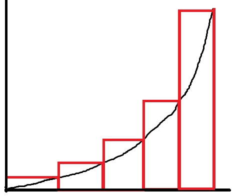
Eventually either a student volunteers (or else I tell the class) that we ought to use a bunch of thin rectangles. For starters, I’ll use five rectangles and a very rough sketch on the board.

I’ll start with the right-most rectangle… what is its area? Students immediately see that the width is $1/5$ , but the length takes a little bit more thought. And I make my students figure it out without me giving them the answer. Eventually, someone notices that the height is simply $f(1) = 1$ , so that the rightmost rectangle has an area of $0.2$ .

I then move to the rectangle that’s second to the right. This also has a width of $1/5$ , but the height is $(0.8)^2 = 0.64$ . So the area is $0.128$ .

Eventually, we get that the sum of the areas is $0.008 + 0.032 + 0.072 + 0.128 + 0.2 = 0.44$ . Students can easily see that this is a decent approximation to the area under the parabola, but it’s a bit too large.

I then ask the same question that I had before: how can we get a better approximation? Students will usually volunteer either “More rectangles” or “Thinner rectangles,” which of course are logically equivalent. I then proceed with 10 equal-width rectangles. Occasionally, a student volunteers that perhaps we should use thinner rectangles only on the right side of the figure, which of course is a very astute observation. However, I tell my class that, for the sake of simplicity, we’ll stick with rectangles of equal width.

With ten rectangles (and I redraw the picture with ten thin rectangles), the approximation is quickly found to be

$0.1 [ (0.1)^2 + (0.2)^2 + \dots + (0.9)^2 + 1^2] = 0.385$

I like using ten rectangles, as that’s probably the largest number that can be handled in class without a calculator (until the very last step of adding up the areas).

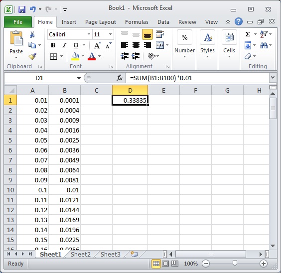
By now, the class sees what the next steps are: take more and more rectangles. At this point, I’ll resort to classroom technology to make the process a little quicker. I personally prefer Microsoft Excel, though other software packages can be used for this purpose. For $100$ rectangles, the class quickly sees that the sum of the rectangles is

$0.01 [ (0.01)^2 + (0.02)^2 + \dots + (0.99)^2 +( 1.00)^2] = 0.33835$

My class can see that the answer is still too large, but it’s certainly closer to the correct answer.

I’ll then tell the class that this is another example of passing to limits, the second theme of calculus. I’ll describe this more fully in the next post.

Day One of my Calculus I class: Part 3

I’ve just told students that the topics in Calculus I build upon each other (unlike the topics of Precalculus), but that there are going to be two themes that run throughout the course:

Approximating curved things by straight things, and
Passing to limits

We are now studying the following problem.

Problem #1. A building on campus is 144 feet tall. A professor takes a particularly annoying student to the top of the building, and throws him (or her) off to his (or her) certain demise. (Usually I pick a student that I know and like as the one to throw off the building. This became a badge of honor over the years.) The distance that the student travels (in feet) after $t$ seconds is $f(t) = 16t^2$ . How fast is the student going when he (or she) hits the concrete sidewalk?

At this point in the lecture, we have done some experimental numerical work with successfully smaller time intervals to find better and better approximations to the speed at impact.

With a time interval of length $3$ seconds, the approximation is $48$ ft/s.
With a time interval of length $1$ seconds, the approximation is $80$ ft/s.
With a time interval of length $0.5$ seconds, the approximation is $88$ ft/s.
With a time interval of length $0.1$ seconds, the approximation is $94.4$ ft/s.
With a time interval of length $0.01$ seconds, the approximation is $95.84$ ft/s.

By this point, students realize that we’re getting better and better approximations… however, we’re probably not going to get the correct answer by just plugging in numbers. And we certainly can’t just take a time interval of $0$ seconds since dividing by zero is a no-no.

Depending on my read of the class — on whether or not they’re ready for a little more abstraction — I’ll then ask the class, “How can we make these fractions without plugging in all of these numbers?” Usually students are at a loss at first. Perhaps someone will volunteer that we ought to introduce a variable… but, in my experience, even bright students at the start of calculus do not have this step of abstraction at the tips of their fingers. So I’ll lay out the fractions that we’ve studied so far, like

$\displaystyle \frac{f(3) - f(2.9)}{0.1} \qquad$ and $\qquad \displaystyle \frac{f(3)-f(2.99)}{0.01}$ ,

and ask, “How could we do this more systematically? Does anyone see a pattern in these fractions?” Hopefully someone will notice that the input of the second function call is 3 minus the denominator; if not, I’ll volunteer this observation to the class. So both of these fractions can be written as

$\displaystyle \frac{f(3) - f(3-h)}{h}$ ,

where $h$ is a small positive number. Let’s now simplify this fraction:

$\displaystyle \frac{f(3) - f(3-h)}{h} = \displaystyle \frac{16(3)^2 - 16(3-h)^2}{h}$

$= \displaystyle \frac{144 - 16(9-6h+h^2)}{h}$

$= \displaystyle \frac{144 - 144 + 96h - 16h^2}{h}$

$= \displaystyle \frac{96h - 16h^2}{h}$

$= \displaystyle 96 - 16h$ .

The last step is permitted because $h$ is assumed to be a nonzero number. I then check to see if the previous work matches this algebraic expression:

If $h=1$ , then $96 - 16h = 80$ , matching the previous answer.
If $h=0.1$ , then $96-16h = 94.8$ , matching the previous answer.

I then ask the class, what’s the ultimate goal with $h$ ? The answer: send $h$ to zero. So we conclude that the velocity at impact is $96 - 16(0) = 96$ ft/s, which is the final answer.

Reviewing, the curved thing was the changing speed of the falling object, which was approximated by the straight thing, the ordinary distance-rate-time formula. Finally, we passed to limits to find the real velocity at impact.

All of the above is eventually done more systematically later in the semester after the properties of derivatives have been more fully developed. However, I think that doing this calculation on the very first day of class gives my students a taste of what’s going to be happening in the days and weeks to come. Again, I emphasize that I probably cover this material in maybe 15-20 minutes, and that I don’t hold students immediately responsible for repeating such a calculation on their own. (I do hold them responsible for this, of course, after they know how to differentiate $f(t) = 16 t^2$ .

Day One of my Calculus I class: Part 2

I’ve just told students that the topics in Calculus I build upon each other (unlike the topics of Precalculus), but that there are going to be two themes that run throughout the course:

Approximating curved things by straight things, and
Passing to limits

I then transition to applying these two themes to two different problems. Here’s the first.

Problem #1. A building on campus is 144 feet tall. A professor takes a particularly annoying student to the top of the building, and throws him (or her) off to his (or her) certain demise. (Usually I pick a student that I know and like as the one to throw off the building. This became a badge of honor over the years.) The distance that the student travels (in feet) after $t$ seconds is $f(t) = 16t^2$ . How fast is the student going when he (or she) hits the concrete sidewalk?

And then I ask my students how to solve this. Usually, they can come up with the first few ideas.

1. When the student hits the sidewalk and meet his/her demise? So we must solve $16t^2 = 144$ , so that $t = \pm 3$ . (And I make sure that they remember that this quadratic equation has two roots.) The solution $t = -3$ is clearly extraneous, so the time elapsed until the student meets his/her demise is $3$ seconds.

2. How fast is the student going after $3$ seconds? Most students realize the inherent difficulty of this question because the student’s speed is increasing as he/she gets closer to the ground. Some students will volunteer the word “accelerate.”

At this point, I’ll volunteer that the changing speed is a curved thing. Back in pre-algebra, students were taught

$\hbox{rate} = \hbox{distance} / \hbox{time}$

under the assumption that the rate was constant. However, if the rate is changing, all bets are off.

Still, the question remains: how fast is the student moving after 3 seconds? How should we measure this? Usually, someone will suggest that we just divide $144$ feet by $3$ seconds, for a rate of $48$ ft/sec. I then point out that this is an example of approximating a curved thing by a straight thing. The straight thing is the usual distance-rate-time formula, while the curved thing is the changing speed of the student as he/she falls. So the answer of $48$ ft/sec is not the correct answer, but it’s an approximate answer.

This leads to the next question: is this estimate too high or too low? Unequivocally, students answer “too low” since the student travels the slowest at the start of the fall and the fastest at the end of the fall. So since this interval of 3 seconds includes the slower speeds at the start of the fall, the answer of $48$ ft/sec will underestimate the speed at impact.

Which then leads to the next obvious question: How can we get a better approximation? I leave the question open-ended like this and take suggestions from the class. This often takes a while, and I’ll get a lot of creative (but bad) ideas. And that’s OK… the next step is hardly the most intuitive thing that immediately jumps to mind. I think that the process of keeping the answer unknown until someone volunteers the correct next step is worth it.

Eventually (though it might take a couple of minutes), somebody will suggest using a shorter time interval, like the distance traveled between $t=2$ and $t=3$ . We see that $f(2) = 64$ and $f(3) = 144$ , and so the new approximation is $(144-64)/1 = 80$ ft/s. I store these two approximations ( $48$ ft/s with a time interval of $3$ seconds and $80$ ft/s with a time interval of $1$ second in a table on the side of the chalkboard. The values derived below are entered in the table as they’re found.

I then note that the previous approximation was $48$ ft/s, and then ask the class, “Do you think that $80$ ft/s will be a better or worse approximation than $48$ ft/s?” Invariably, they’ll say it’s a better approximation because the change in speed isn’t as great from $t=2$ to $t=3$ as from $t=0$ to $t=3$ . I’ll then ask if they think that $80$ ft/s is too high or too low. Again, they’ll answer too low for the same reason as before.

Then I ask the obvious next question, “How do we find a better approximation?” The class typically responds something to the effect of, “Take a smaller interval.” I ask for a suggestion, and I’ll usually get something like $t=2.5$ to $t=3$ . We see that $f(2.5)=100$ ft/s and $f(3)$ is still $144$ ft/s, so that the new approximation is $(144-100)/0.5 = 88$ ft/s. Students will volunteer that this should be better than the previous two approximations but still less than the correct answer.

Then I do it again: “How do we find a better approximation?” The class typically respond, “Take an even smaller interval.” I suggest $t=2.9$ to $t=3$ . We see that $f(2.9)=134.56$ ft/s (by this point, a calculator is certainly needed) and $f(3)$ is still $144$ ft/s, so that the new approximation is $(144-134.56)/0.1 = 94.4$ ft/s. If we do it again with $t =2.99$ , we see that $f(2.99) =143.0416$ ft/s, for an approximation of $(144-143.0416)/0.01 = 95.84$ ft/s.

I turn to the class and ask, “Have we found the right answer yet?” They’ll answer “No” in unison, but they’ll note that the approximations are probably pretty good right now. Astute students will notice that the approximations appear to be “leveling off” to some final value.

I’ll then tell the class that this is an example of passing to limits, the second theme of calculus. By making the time intervals smaller and smaller, we get better and better approximations to the true speed at impact. In the next post, I’ll describe how I informally introduce the concept of a limit with this example.

Day One of my Calculus I class: Part 1

I begin by noting the different topics that appear in Precalculus, which they should have taken in the recent past:

The definition of a function and an inverse function
Graphing polynomials and rational functions
Properties and applications of exponential and logarithmic functions
Trigonometry
Sequences and series

These different topics, when taught in Precalculus, really don’t talk to one another. With a couple of exceptions, it feels like five different units being squeezed into the same course. I’ll present a visual image of laying down an imaginary brick on the floor, and then laying down a second brick next to the first one, and so on. The above topics (with a couple of exceptions) really don’t build upon each other; they’re lateral to one another. In other words, these topics made the foundation necessary for the study of calculus. After all, the class was called Pre-Calculus.

Now that we’re in calculus, I tell my students, we’re going to have topics that build on this foundation, and the topics will build on each other. Continuing the building image, I’ll start laying imaginary bricks on the initial foundation, building vertically higher and higher, noting that the topics that we’ll see in Weeks 13 and 14 will ultimately be built upon the topics that we’ll talk about in Weeks 1 and 2. Unlike Precalculus, the topics in Calculus are explicitly interconnected, building up a body of thought from the foundation of Precalculus.

So the good news is that, unlike Precalculus, Calculus I will be an incrementally developed course from start to finish. The bad news, of course, is that Calculus I will be an incrementally developed course from start to finish. In Precalculus, if you didn’t particularly like one topic (say, logarithms), that really would not affect your success later on with a future topic (say, trigonometry). However, in Calculus, the whole course is put together from start to finish.

The good news is that while there are many interconnected topics in calculus, there are going to be two themes that run throughout the course:

Approximating curved things by straight things, and
Passing to limits

And we’re going to be applying these two themes again and again throughout the semester. (I wish I could take credit for synthesizing the topics of calculus into these two themes, but I learned this idea from my own calculus professor back in the mid-1980s.)

For the remainder of this first lecture, I show how these two themes apply to two completely different problems:

Finding the speed of a falling object when it hits the ground.
Finding the area under the curve $y = x^2$ between $x = 0$ and $x = 1$ .

I’ll describe how I present these to new calculus students in the coming posts.

Area of a circle (Part 3)

Math majors are completely comfortable with the formula $A = \pi r^2$ for the area of a circle. However, they often tell me that they don’t remember a proof or justification for why this formula is true. And they certainly don’t remember a justification that would be appropriate for showing geometry students.

$A = \displaystyle \iint_R 1 \, dx \, dy$

This double integral may be computed by converting to polar coordinates. The distance from the origin varies from $r=0$ to $r=a$ , while the angle varies from $\theta = 0$ to $\theta = 2\pi$ . Using the conversion $dx \, dy = r \, dr \, d\theta$ , we see that

$A = \displaystyle \int_0^{2 \pi} \int_0^a r \, dr \, d \theta$

$A = \displaystyle \int_0^{2\pi} \left[ \frac{r^2}{2} \right]_0^a \, d\theta$

$A = \displaystyle \int_0^{2\pi} \frac{a^2}{2} \, d\theta$

$A = \displaystyle 2 \pi \cdot \frac{a^2}{2}$

$A = \displaystyle \pi a^2$

We note that the above proof uses the fact that calculus with trigonometric functions must be done with radians and not degrees. In other words, we had to change the range of integration to $[0,2\pi]$ and not $[0^o, 360^o]$ .

Area of a circle (Part 2)

A circle centered at the origin with radius $r$ may be viewed as the region between $f(x) = -\sqrt{r^2 - x^2}$ and $g(x) = \sqrt{r^2 - x^2}$ . These two functions intersect at $x = r$ and $x = -r$ . Therefore, the area of the circle is the integral of the difference of the two functions:

$A = \displaystyle \int_{-r}^r \left[g(x) - f(x) \right] \, dx= \displaystyle \int_{-r}^r 2 \sqrt{r^2 - x^2} \, dx$

This may be evaluated by using the trigonometric substitution $x = r \sin \theta$ and changing the range of integration to $\theta = -\pi/2$ to $\theta = \pi/2$ . Since $dx = r \cos \theta \, d\theta$ , we find

$A = \displaystyle \int_{-\pi/2}^{\pi/2} 2 \sqrt{r^2 - r^2 \sin^2 \theta} \, r \cos \theta d\theta$

$A = \displaystyle \int_{-\pi/2}^{\pi/2} 2 r^2 \cos^2 \theta d\theta$

$A = \displaystyle r^2 \int_{-\pi/2}^{\pi/2} (1 + \cos 2\theta) d\theta$

$A = \displaystyle r^2 \left[ \theta + \frac{1}{2} \sin 2\theta \right]_{-\pi/2}^{\pi/2}$

$A = \displaystyle r^2 \left[ \left( \displaystyle \frac{\pi}{2} + \frac{1}{2} \sin \pi \right) - \left( - \frac{\pi}{2} + \frac{1}{2} \sin (-\pi) \right) \right]$

$A = \pi r^2$

Area of a circle (Part 1)

In this series of posts, I’ll discuss several ways that the area of a circle can be found using calculus. I’ll also discuss a straightforward classroom activity by which students can discover for themselves why $A = \pi r^2$ .In the first few weeks after a calculus class, after students are introduced to the concept of limits, the derivative is introduced for the first time… often as the slope of a tangent line to the curve. Here it is: if $y = f(x)$, then

$\displaystyle \frac{dy}{dx} = y' = f'(x) = \lim_{h \to 0} \displaystyle \frac{f(x+h) - f(x)}{h}$

From this definition, the first few rules of differentiation are derived in approximately the following order:

1. If $f(x) = c$ , a constant, then $\displaystyle \frac{d}{dx} (c) = 0$ .

2. If $f(x)$ and $g(x)$ are both differentiable, then $(f+g)'(x) = f'(x) + g'(x)$ .

3. If $f(x)$ is differentiable and $c$ is a constant, then $(cf)'(x) = c f'(x)$ .

4. If $f(x) = x^n$ , where $n$ is a nonnegative integer, then $f'(x) = n x^{n-1}$ . This may be proved by at least two different techniques:

The binomial expansion $(x+h)^n = x^n + n x^{n-1} h + \displaystyle {n \choose 2} x^{n-2} h^2 + \dots + h^n$
The Product Rule (derived later) and mathematical induction

5. If $f(x) = a_n x^n + a_{n-1} x^{n-1} + \dots + a_1 x + a_0$ is a polynomial, then $f'(x) = n a_n x^{n-1} + (n-1) a_{n-1} x^{n-2} + a_1$ . In other words, taking the derivative of a polynomial is easy.

After doing a few examples to help these concepts sink in, I’ll show the following two examples with about 3-4 minutes left in class.

Example 1. Let $A(r) = \pi r^2$ . Notice I’ve changed the variable from $x$ to $r$ , but that’s OK. Does this remind you of anything? (Students answer: the area of a circle.) What’s the derivative? Remember, $\pi$ is just a constant. So $A'(r) = \pi \cdot 2r = 2\pi r$ . Does this remind you of anything? (Students answer: Whoa… the circumference of a circle.)

Example 2. Now let’s try $V(r) = \displaystyle \frac{4}{3} \pi r^3$ . Does this remind you of anything? (Students answer: the volume of a sphere.) What’s the derivative? Again, $\displaystyle \frac{4}{3} \pi$ is just a constant. So $V'(r) = \displaystyle \frac{4}{3} \pi \cdot 3r^2 = 4\pi r^2$ . Does this remind you of anything? (Students answer: Whoa… the surface area of a sphere.)

Hmmm. That’s interesting. The derivative of the area of a circle is the circumference of the circle, and the derivative of the area of a sphere is the surface area of the sphere. I wonder why this works. Any ideas? (Students: stunned silence.)

This is what’s known on television as a cliff-hanger, and I’ll give you the answer at the start of class tomorrow. (Students groan, as they really want to know the answer immediately.)

In the spirit of a cliff-hanger, I offer the following thought bubble before presenting the answer.

By definition, if $A(r) = \pi r^2$ , then

$A'(r) = \displaystyle \lim_{h \to 0} \frac{ A(r+h) - A(r) }{h} = 2\pi r$

The numerator may be viewed as the area of the ring between concentric circles with radii $r$ and $r+h$ . In other words, imagine starting with a solid red disk of radius $r +h$ and then removing a solid white disk of radius $r$ . The picture would look something like this:

Notice that the ring has a thickness of $r+h -r = h$ . If this ring were to be “unpeeled” and flattened, it would approximately resemble a rectangle. The height of the rectangle would be $h$ , while the length of the rectangle would be the circumference of the circle. So

$A(r + h) - A(r) \approx 2 \pi r h$

and we can conclude that

$A'(r) = \displaystyle \lim_{h \to 0} \frac{ 2 \pi r h}{h} = 2\pi r$

By the same reasoning, the derivative of the volume of a sphere ought to be the surface area of the sphere.

Pedagogically, I find that the above discussion helps reinforce the definition of a derivative at a time when students are most willing to forget about the formal definition in favor of the various rules of differentiation.

In the above work, we started with the formula for the area of the circle and then confirmed that its derivative matched the expected result. However, the above logic can be used to derive the formula for the area of a circle from the formula $C(r) = 2\pi r$ for the circumference. We begin with the observation that $A'(r) = C(r)$ , as above. Therefore, by the Fundamental Theorem of Calculus,

$A(r) - A(0) = \displaystyle \int_0^r C(t) \, dt$

$A(r) - A(0) = \displaystyle \int_0^r 2\pi t \, dt$

$A(r) - A(0) = \displaystyle \left[ \pi t^2 \right]_0^r$

$A(r) - A(0) = \pi r^2$

Since the area of a circle with radius $0$ is $0$ , we conclude that $A(r) = \pi r^2$ .

Pedagogically, I don’t particularly recommend this approach, as I think students would find this explanation more confusing than the first approach. However, I can see that this could be useful for reinforcing the statement of the Fundamental Theorem of Calculus.

By the way, the above reasoning works for a square or cube also, but with a little twist. For a square of side length $s$ , the area is $A(s) = s^2$ and the perimeter is $P(s) = 4s$ , which isn’t the derivative of $A(s)$ . The reason this didn’t work is because the side length $s$ of a square corresponds to the diameter of a circle, not the radius of a circle.

But, if we let $x$ denote half the side length of a square, then the above logic works out since

$A(x) = s^2 = (2x)^2 = 4x^2$

and

$P(x) = 4s = 4(2x) = 8x$

Written in terms of the half-sidelength $x$ , we see that $A'(x) = P(x)$ .

Why do we teach students about radians?

Throughout grades K-10, students are slowly introduced to the concept of angles. They are told that there are $90$ degrees in a right angle, $180$ degrees in a straight angle, and a circle has $60$ degrees. They are introduced to $30-60-90$ and $45-45-90$ right triangles. Fans of snowboarding even know the multiples of $180$ degrees up to $1440$ or even $1620$ degrees.

Then, in Precalculus, we make students get comfortable with $\pi$ , $\displaystyle \frac{\pi}{2}$ , $\displaystyle \frac{\pi}{3}$ , $\displaystyle \frac{\pi}{4}$ , $\displaystyle \frac{\pi}{6}$ , and multiples thereof.

We tell students that radians and degrees are just two ways of measuring angles, just like inches and centimeters are two ways of measuring the length of a line segment.

Still, students are extremely comfortable with measuring angles in degrees. They can easily visualize an angle of $75^o$ , but to visualize an angle of $2$ radians, they inevitably need to convert to degrees first. In his book Surely You’re Joking, Mr. Feynman!, Nobel-Prize laureate Richard P. Feynman described himself as a boy:

I was never any good in sports. I was always terrified if a tennis ball would come over the fence and land near me, because I never could get it over the fence – it usually went about a radian off of where it was supposed to go.

Naturally, students wonder why we make them get comfortable with measuring angles with radians.

The short answer, appropriate for Precalculus students: Certain formulas are a little easier to write with radians as opposed to degrees, which in turn make certain formulas in calculus a lot easier.

The longer answer, which Precalculus students would not appreciate, is that radian measure is needed to make the derivatives of $\sin x$ and $\cos x$ look palatable.

Source: http://mathworld.wolfram.com/CircularSector.html

1. In Precalculus, the length of a circle arc with central angle $\theta$ in a circle with radius $r$ is

$s = r\theta$

Also, the area of a circular sector with central angle $\theta$ in a circle with radius $r$ is

$A = \displaystyle \frac{1}{2} r^2 \theta$

In both of these formulas, the angle $\theta$ must be measured in radians.

Students may complain that it’d be easy to make a formula of $\theta$ is measured in degrees, and they’d be right:

$s = \displaystyle \frac{180 r \theta}{\pi}$ and $A = \displaystyle \frac{180}{\pi} r^2 \theta$

However, getting rid of the $180/\pi$ makes the following computations from calculus a lot easier.

2a. Early in calculus, the limit

$\displaystyle \lim_{\theta \to 0} \frac{\sin \theta}{\theta} = 1$

is derived using the Sandwich Theorem (or Pinching Theorem or Squeeze Theorem). I won’t reinvent the wheel by writing out the proof, but it can be found here. The first step of the proof uses the formula for the above formula for the area of a circular sector.

2b. Using the trigonometric identity $\cos 2x = 1 - 2 \sin^2 x$ , we replace $x$ by $\theta/2$ to find

$\displaystyle \lim_{\theta \to 0} \frac{1 - \cos \theta}{\theta} = \displaystyle \lim_{\theta \to 0} \frac{2\sin^2 \displaystyle \left( \frac{\theta}{2} \right)}{ \theta}$

$\displaystyle \lim_{\theta \to 0} \frac{1 - \cos \theta}{\theta} = \displaystyle \lim_{\theta \to 0} \sin \left( \frac{\theta}{2} \right) \cdot \frac{\sin \displaystyle \left( \frac{\theta}{2} \right)}{ \displaystyle \frac{\theta}{2}}$

$\displaystyle \lim_{\theta \to 0} \frac{1 - \cos \theta}{\theta} =0 \cdot 1$

$\displaystyle \lim_{\theta \to 0} \frac{1 - \cos \theta}{\theta} =0$

3. Both of the above limits — as well as the formulas for $\sin(\alpha + \beta)$ and $\cos(\alpha + \beta)$ — are needed to prove that $\displaystyle \frac{d}{dx} \sin x = \cos x$ and $\displaystyle \frac{d}{dx} \cos x = -\sin x$ . Again, I won’t reinvent the wheel, but the proofs can be found here.

So, to make a long story short, radians are used to make the derivatives $y = \sin x$ and $y = \cos x$ easier to remember. It is logically possible to differentiate these functions using degrees instead of radians — see http://www.math.ubc.ca/~feldman/m100/sinUnits.pdf. However, possible is not the same thing as preferable, as calculus is a whole lot easier without these extra factors of $\pi/180$ floating around.