Thoughts on Numerical Integration (Part 5): Derivation of Simpson’s Rule

Numerical integration is a standard topic in first-semester calculus. From time to time, I have received questions from students on various aspects of this topic, including:

Why is numerical integration necessary in the first place?
Where do these formulas come from (especially Simpson’s Rule)?
How can I do all of these formulas quickly?
Is there a reason why the Midpoint Rule is better than the Trapezoid Rule?
Is there a reason why both the Midpoint Rule and the Trapezoid Rule converge quadratically?
Is there a reason why Simpson’s Rule converges like the fourth power of the number of subintervals?

In this series, I hope to answer these questions. While these are standard questions in a introductory college course in numerical analysis, and full and rigorous proofs can be found on Wikipedia and Mathworld, I will approach these questions from the point of view of a bright student who is currently enrolled in calculus and hasn’t yet taken real analysis or numerical analysis.

In the previous post in this series, I discussed three different ways of numerically approximating the definite integral $\displaystyle \int_a^b f(x) \, dx$ , the area under a curve $f(x)$ between $x=a$ and $x=b$ .

In this series, we’ll choose equal-sized subintervals of the interval $[a,b]$ . If $h = (b-a)/n$ is the width of each subinterval so that $x_k = x_0 + kh$ , then the integral may be approximated as

$\int_a^b f(x) \, dx \approx h \left[f(x_0) + f(x_1) + \dots + f(x_{n-1}) \right] \equiv L_n$

using left endpoints,

$\int_a^b f(x) \, dx \approx h \left[f(x_1) + f(x_2) + \dots + f(x_n) \right] \equiv R_n$

using right endpoints, and

$\int_a^b f(x) \, dx \approx h \left[f(c_1) + f(c_2) + \dots + f(c_n) \right] \equiv M_n$

using the midpoints of the subintervals. We have also derived the Trapezoid Rule:

$\int_a^b f(x) \, dx \approx \displaystyle \frac{h}{2} [f(x_0) + 2f(x_1) + \dots + 2f(x_{n-1}) + f(x_n)] \equiv T_n$

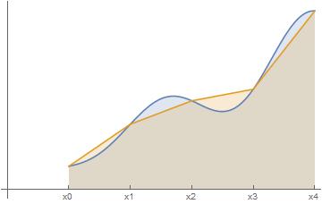
This last approximation was obtained by connecting adjacent points on the curve by line segments, creating trapezoids:

In this post, we will derive Simpson’s Rule. Instead of connecting two adjacent points with line segments, we will connect three adjacent points with a parabola. In the picture below, the points $(x_0, f(x_0))$ , $(x_1, f(x_1))$ and $(x_2,f(x_2))$ are connected with one parabola, while the points $(x_2, f(x_2))$ , $(x_3, f(x_3))$ and $(x_4,f(x_4))$ are connected with a different second parabola.

Clearly, for this to work, there has to be an even number of subintervals. (By contrast, for the Trapezoid Rule, the Midpoint Rule, or the endpoint rules, the number of subintervals could be even or odd.)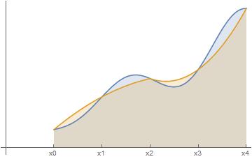

The derivation of Simpson’s Rule is more complicated than the derivation of the Trapezoid Rule because we need to use calculus to find the area under these parabolas. To begin, we make the simplifying assumption that $x_1 = 0$ . Since each subinterval has width $h$ , this means that $x_0 = -h$ and $x_2 = h$ .

To find the area under this parabola, we first need to find the equation of the parabola $y = ax^2 + bx + c$ connecting the three points $(-h,y_0)$ , $(0,y_1)$ , and $(h,y_2)$ . This entails solving a system of three equations in three unknowns:

$a(-h)^2 + b(-h) + c = y_0$

$a(0)^2+b(0) + c = y_1$

$ah^2 + bh + c = y_2$ ,

$ah^2 - bh + c = y_0$

$c = y_1$

$ah^2 + bh + c = y_2$ .

While most 3×3 systems are cumbersome to solve, this system is straightforward. Clearly, $c = y_1$ . Also, subtracting the first equation from the third equation yields

$2bh = y_2 - y_0$ , or $b = \displaystyle \frac{y_2 - y_0}{2h}$

Finally, we solve for $a$ by substituting into the third equation:

$ah^2 + \displaystyle \frac{y_2 - y_0}{2h} h + y_1 = y_2$

$ah^2 + \displaystyle \frac{y_2 - y_0}{2} + y_1 = y_2$

$ah^2 = \displaystyle \frac{y_0 - y_2}{2} - \frac{2y_1}{2} + \frac{2y_2}{2}$

$ah^2 = \displaystyle \frac{y_0 - 2y_1 + y_2}{2}$

$a = \displaystyle \frac{y_0 - 2y_1 + y_2}{2h^2}$

Next, we find the integral of $y = ax^2 + bx + c$ between $x = -h$ and $x = h$ :

$\displaystyle \int_{-h}^h (ax^2 + bx + c) \, dx = \left[ \frac{ax^3}{3} + \frac{bx^2}{2} + cx \right]^h_{-h}$

$= \displaystyle \left[ \frac{ah^3}{3} + \frac{bh^2}{2} + ch \right] - \left[ -\frac{ah^3}{3} + \frac{bh^2}{2} - ch \right]$

$= \displaystyle \frac{2ah^3}{3} + 2ch$

$= \displaystyle \frac{(y_0 - 2y_1 + y_2)h}{3} + 2y_1h$

$= \displaystyle \frac{h(y_0 + 4y_1 + y_2)}{3}$ .

We now turn to the more general case of finding the area under the parabola passing through $(x_0,y_0)$ , $(x_1,y_1)$ , and $(x_2,y_2)$ , where $x_1 = x_0 +h$ and $x_2 = x_1 + 2h$ . Geometrically, it should be clear that this parabola can be obtained from the above parabola by a horizontal translation. Since the area under the curve is not changed by a horizontal translation, the area (and the formula) will be the same.

More formally, if $y = ax^2 + bx + c$ passes through the points $(-h,y_0)$ , $(0,y_1)$ , and $(h,y_2)$ , then $y = a(x-x_1)^2 + b(x-x_1) + c$ will pass through the points $(x_0,y_0)$ , $(x_1,y_1)$ , and $(x_2,y_2)$ . The area under this curve is

$\displaystyle \int_{x_0}^{x_2} \left[ a(x-x_1)^2 + b(x-x_1) + c \right] \, dx$ .

After using the substitution $u = x-x_1$ , this becomes

$\displaystyle \int_{-h}^h (au^2 + bu + c) \, du$ ,

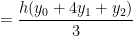
which is the same integral that we saw earlier. Therefore,

$\displaystyle \int_{x_0}^{x_2} \left[ a(x-x_1)^2 + b(x-x_1) + c \right] \, dx = \displaystyle \frac{h(y_0 + 4y_1 + y_2)}{3}$ .

Finally, we need to find the sum of the areas under all of these parabolas. Similarly, the area under the parabola passing through $(x_2,y_2)$ , $(x_3,y_3)$ , and $(x_4,y_4)$ will be $\displaystyle \frac{h(y_2 + 4y_3 + y_4)}{3}$ . So, for the particular example shown above, the total area under the parabolas will be

$\displaystyle \frac{h(y_0 + 4y_1 + y_2)}{3} + \frac{h(y_2 + 4y_3 + y_4)}{3} = \frac{h}{3} (y_0 + 4 y_1 + 2 y_2 + 4 y_3 + y_4)$ .

The coefficients of 4 arose from the above integrals, while the coefficient of 2 came from combining the two areas. In general, if there are $n$ subintervals and $n$ is even, then Simpson’s Rule gives the approximation

$S_n = \displaystyle \frac{h}{3} \left(y_0 + 4 y_1 + 2 y_2 + 4 y_3 + \dots + 2y_{n-2} + 4 y_{n-1} + y_{n} \right)$ .

Thoughts on Numerical Integration (Part 4): Derivation of Trapezoid Rule

Numerical integration is a standard topic in first-semester calculus. From time to time, I have received questions from students on various aspects of this topic, including:

Why is numerical integration necessary in the first place?
Where do these formulas come from (especially Simpson’s Rule)?
How can I do all of these formulas quickly?
Is there a reason why the Midpoint Rule is better than the Trapezoid Rule?
Is there a reason why both the Midpoint Rule and the Trapezoid Rule converge quadratically?
Is there a reason why Simpson’s Rule converges like the fourth power of the number of subintervals?

In this series, we’ll choose equal-sized subintervals of the interval $[a,b]$ . If $h = (b-a)/n$ is the width of each subinterval so that $x_k = x_0 + kh$ , then the integral may be approximated as

$\int_a^b f(x) \, dx \approx h \left[f(x_0) + f(x_1) + \dots + f(x_{n-1}) \right] \equiv L_n$

using left endpoints,

$\int_a^b f(x) \, dx \approx h \left[f(x_1) + f(x_2) + \dots + f(x_n) \right] \equiv R_n$

using right endpoints, and

$\int_a^b f(x) \, dx \approx h \left[f(c_1) + f(c_2) + \dots + f(c_n) \right] \equiv M_n$

using the midpoints of the subintervals.

All three of these approximations were obtained by approximating the above shaded region by rectangles. However, perhaps it might be better to use some other shape besides rectangles. In the Trapezoidal Rule, we approximate the area by using (surprise!) trapezoids, as in the figure below.

The first trapezoid has height $h$ and bases $f(x_0)$ and $f(x_1)$ , and so the area of the first trapezoid is $\frac{1}{2} h[ f(x_0) + f(x_1) ]$ . The other areas are found similarly. Adding these together, we get the approximation

$T_n = \displaystyle \frac{h}{2}[f(x_0) + f(x_1)] + \frac{h}{2} [f(x_1) + f(x_2)] + \dots +$

$+ \displaystyle \frac{h}{2} [f(x_{n-2})+f(x_{n-1})] + \frac{h}{2} [f(x_{n-1})+f(x_n)]$

$= \displaystyle \frac{h}{2} [f(x_0) + 2f(x_1) + 2f(x_2) + \dots + 2f(x_{n-2}) + 2f(x_{n-1}) + f(x_n)].$

Interestingly, $T_n$ is the average of the two endpoint approximations $L_n$ and $R_n$ :

$\displaystyle \frac{L_n+R_n}{2} = \frac{L_n}{2} + \frac{R_n}{2}$

$= \displaystyle \frac{h}{2} \left[f(x_0) + f(x_1) + f(x_2) + \dots + f(x_{n-1}) \right]$

$+\displaystyle \frac{h}{2} \left[f(x_1) + f(x_2) + \dots + f(x_{n-1}) + f(x_{n}) \right]$

$= \displaystyle \frac{h}{2} \left[f(x_0) + 2f(x_1) + \dots + 2f(x_{n-1}) + f(x_n) \right]$

$= T_n$ .

Of course, as a matter of computation, it’s a lot quicker to directly compute $T_n$ instead of computing $L_n$ and $R_n$ separately and then averaging.

Thoughts on Numerical Integration (Part 3): Derivation of left, right, and midpoint rules

Numerical integration is a standard topic in first-semester calculus. From time to time, I have received questions from students on various aspects of this topic, including:

Why is numerical integration necessary in the first place?
Where do these formulas come from (especially Simpson’s Rule)?
How can I do all of these formulas quickly?
Is there a reason why the Midpoint Rule is better than the Trapezoid Rule?
Is there a reason why both the Midpoint Rule and the Trapezoid Rule converge quadratically?
Is there a reason why Simpson’s Rule converges like the fourth power of the number of subintervals?

For the sake of completeness, I discuss here the origins of the left-endpoint, right-endpoint, and midpoint rules of numerical integration. (These topics are often presented in calculus texts.) Consider the problem of finding $\displaystyle \int_a^b f(x) \, dx$, the area under a curve $f(x)$ between $x=a$ and $x=b$ .

To start the process of numerical integration, the interval $[a,b]$ is divided into subintervals. Usually, for convenience, the intervals are chosen to be the same length, a convention that I’ll follow in this series. That said, if the function is known to vary wildly on some parts of the domain but not so wildly on other parts, then computational efficiency can be gained by varying the sizes of the subintervals, choosing smaller subintervals for the places where the function varies wildly.

In any event, we’ll choose equal-sized subintervals for the duration of this series.

One numerical approximation can be made by choosing left endpoints. In the picture below, the interval $[a,b]$ was divided into four equal subintervals. Let $h = (b-a)/4$ , so that $x_0 = a$ , $x_1 = x_0 +h$ , $x_2 = x_0 + 2h$ , $x_3 = x_0 + 3h$ , and $x_4 = x_0 + 4h = b$ . We then can draw rectangles using the left endpoints of each subinterval. The sum of the areas of these rectangles below is

$hf(x_0) + hf(x_1) + hf(x_2) +hf(x_3)$ ,

and so this serves as an approximation to the area under the curve. In general, if there are $n$ subintervals and $x_k = x_0 + kh$ , then the integral may be approximated as

$\int_a^b f(x) \, dx \approx h \left[f(x_0) + f(x_1) + \dots + f(x_{n-1}) \right]$

That said, left endpoints were not necessary for making an approximation. We could have instead chosen the right endpoints of each subinterval. The sum of the areas of the rectangles below is

$hf(x_1) + hf(x_2) + hf(x_3) +hf(x_4)$ ,

and so this serves as an approximation to the area under the curve. In general, if there are $n$ subintervals, then the integral may be approximated as

$\int_a^b f(x) \, dx \approx h \left[f(x_1) + f(x_2) + \dots + f(x_n) \right]$

As a final approximation, any point in each subinterval could’ve been used for making an approximation. In the picture below, we use the midpoints of the subintervals, where $c_k = (x_k + x_{k-1})/2$ . The sum of the areas of the rectangles below is

$hf(c_1) + hf(c_2) + hf(c_3) +hf(c_4)$ ,

and so this serves as an approximation to the area under the curve. In general, if there are $n$ subintervals, then the integral may be approximated as

$\int_a^b f(x) \, dx \approx h \left[f(c_1) + f(c_2) + \dots + f(c_n) \right]$

Thoughts on Numerical Integration (Part 2): The bell curve

Numerical integration is a standard topic in first-semester calculus. From time to time, I have received questions from students on various aspects of this topic, including:

Why is numerical integration necessary in the first place?
Where do these formulas come from (especially Simpson’s Rule)?
How can I do all of these formulas quickly?
Is there a reason why the Midpoint Rule is better than the Trapezoid Rule?
Is there a reason why both the Midpoint Rule and the Trapezoid Rule converge quadratically?
Is there a reason why Simpson’s Rule converges like the fourth power of the number of subintervals?

In this post, I’d like to take a closer look at the indefinite integral $\displaystyle \int e^{-x^2} dx$ , which is closely related to the area under the bell curve $\displaystyle \frac{1}{\sqrt{2\pi}} e^{-x^2/2} dx$ . This integral cannot be computed using elementary functions. However, using integration by parts, there are some related integrals that can be computed:

$\displaystyle \int x e^{-x^2} dx = -\displaystyle \frac{1}{2} e^{-x^2}$

$\displaystyle \int x^3 e^{-x^2} dx = -\displaystyle \frac{x^2+1}{2} e^{-x^2}$

$\displaystyle \int x^5 e^{-x^2} dx = -\displaystyle \frac{x^4+2x^2+2}{2} e^{-x^2}$

$\displaystyle \int x^7 e^{-x^2} dx = -\displaystyle \frac{x^6+3x^4+6x^2+6}{2} e^{-x^2}$

Based on these examples, it stands to reason that, if $\displaystyle \int e^{-x^2} dx$ can be written in terms of elementary functions, it should have the form

$\displaystyle \int e^{-x^2} dx = f(x) e^{-x^2}$ ,

where $f(x)$ is some polynomial to be determined. We will now show that this is impossible.

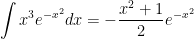
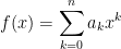Suppose $f(x) = \displaystyle \sum_{k=0}^n a_k x^k$ , a polynomial of degree $n$ to be determined. Then we have

$\displaystyle \frac{d}{dx} \left[ f(x) e^{-x^2} \right] = e^{-x^2}$

$f'(x) e^{-x^2} - 2 x f(x) e^{-x^2} =e^{-x^2}$

$f'(x) - 2x f(x) = 1$ .

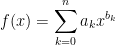In other words, all terms on the left-hand side except the constant term must cancel. However, this is impossible: $2x f(x)$ is a polynomial of degree $n+1$ while $f'(x)$ is a polynomial of degree $n-1$ . Therefore, the left hand side must have degree $n+1$ and therefore cannot be a constant.

A similar argument shows that $f(x)$ cannot have the form $f(x) = \displaystyle \sum_{k=0}^n a_k x^{b_k}$ , where the exponents $b_k$ may or may not be integers.

This may be enough to convince a calculus student that there is no elementary antiderivative of $\displaystyle e^{-x^2} dx$ . Indeed, although the proof goes well beyond first-year calculus, there is a theorem that says that if $\displaystyle \int x^a e^{bx^2}$ can be expressed in terms of elementary functions, then the antiderivative must have the form $f(x) e^{b x^2}$ . So the guess above actually can be rigorously justified. References:

Elena Anne Marchisotto and Gholam-Ali Zakeri, “An Invitation to Integration in Finite Terms,” The College Mathematics Journal , Sep., 1994, Vol. 25, No. 4 (Sep., 1994), pp. 295-308
J. F. Ritt, Integration in Finite Terms: Liouville’s Theory of Elementary Methods, Columbia University Press, New York, 1948

Thoughts on Numerical Integration (Part 1): Why numerical integration?

Numerical integration is a standard topic in first-semester calculus. From time to time, I have received questions from students on various aspects of this topic, including:

Why is numerical integration necessary in the first place?
Where do these formulas come from (especially Simpson’s Rule)?
How can I do all of these formulas quickly?
Is there a reason why the Midpoint Rule is better than the Trapezoid Rule?
Is there a reason why both the Midpoint Rule and the Trapezoid Rule converge quadratically?
Is there a reason why Simpson’s Rule converges like the fourth power of the number of subintervals?

First, let’s talk about why numerical integration is necessary in the first place. Indeed, I can still remember a high school calculus teacher asking me this question nearly 20 years ago, and this question really got me thinking about what we’re collectively teaching in the secondary curriculum. Indeed, in a Calculus I course, it seems like every integral can be computed if only the proper trick is used. We teach students to search for these different tricks:

Let $u = x^2+5$ to find $\displaystyle \int \frac{6x \, dx}{\sqrt{x^2+9}}$ .
Let $x = 3\tan \theta$ to find $\displaystyle \int \frac{6 \, dx}{\sqrt{x^2+9}}$
Use integration by parts to find $\displaystyle \int x^3 e^x \, dx$

In fact, we teach so many tricks that we may give the impression that every integral can be computed if only the proper trick is employed. Indeed, my university hosts an annual “Integration Bee” that challenges students to find the right technique(s) to evaluate some pretty tough integrals.

Unfortunately, not every integral can be solved in terms of a finite number of elementary functions (polynomials, rational functions, exponential functions, logarithms, trigonometric and inverse trigonometric functions). One function that is commonly known to many students which does not have an elementary antiderivative is $\displaystyle \frac{1}{\sqrt{2\pi}} e^{-x^2/2}$ , otherwise known as the bell curve. For most numbers $a$ and $b$ , the area

$\displaystyle \int_a^b \frac{1}{\sqrt{2\pi}} e^{-x^2/2}$

cannot be found exactly, and so we ask students to either use a table in the back of the textbook or else use a function on their scientific calculators to find the answer.

Just for the fun of it, I went through my Ph.D. thesis and wrote down some of the integrals that I had to integrate numerically while in school. As an applied mathematician, I was initially stunned by the teacher’s innocent question because so much of my work would be utterly impossible if it wasn’t for numerical integration. Here are some of the easier ones:

$\displaystyle \int_0^t \frac{1-e^{-x}}{x} dx$
$\displaystyle \int_{2R}^\infty t^2 g(t) \left( \frac{a_1 t^4 + a_2 t^2 + a_3}{(t^2-R^2)^7} +\frac{b_1 t^2 + b_2}{(t^2-R^2)^5} + \frac{c}{(t^2-R^2)^3} \right) dt$
$\displaystyle \int_{d_2}^\infty \int_0^{d_1} \frac{y^2-x^2}{(x^2+y^2)^2} \left(e^{-a(x+d_1)-b d_2} - c\right) dx \, dy$
$\displaystyle \int_{x/2}^\infty \sqrt{r^2 - k^2/4} \phi(r) \, dr$
$\displaystyle \int_{x/2}^\infty \left( \frac{z \sqrt{4r^2-z^2}}{4} + r^2 \arcsin \left( \frac{z}{2r} \right) \right) \phi(r) \, dr$
$\displaystyle \int_0^{2R} e^{-sz} \exp \left[ -c \left( z \sqrt{4R^2-z^2} + 4R^2 \arcsin \frac{z}{2R} \right) \right] dz$
$\displaystyle \int_0^d \exp \left[ -sz - \lambda \left(z - \frac{z^2}{4d} \right) \right] dz$
$\displaystyle \int_d^{d \sqrt{2}} \exp \left[ -sz - \lambda \left( \frac{d (\pi+1)}{2} - d \arcsin \frac{d}{z} + \frac{z^2}{4d} - \sqrt{z^2-d^2} \right) \right] dz$
$\displaystyle \int_0^\infty \exp \left[-sz - \eta \left(1 - e^{-cz/2} - \frac{cz}{4} e^{-cz/2} \right) \right] dz$
$\displaystyle \int_{-\infty}^x \frac{e^t}{t} dt$

All this to say, there are plenty of integrals that arise from a real-world context that have a numerical answer but cannot be computed using the techniques commonly taught in the first-year calculus sequence.

Terrific video on Taylor series

Some time ago, I posted a series on the lecture that I’ll give to student to remind them about Taylor series. I won’t repost the whole thing here, but the basic ideas are inductively motivating the concept by starting with a polynomial and then reinforcing the concept with both numerical calculation and comparison of graphs.

After giving this lecture recently, one of my students told me about this terrific video on Taylor series that does much of the same things, with the added bonus of engaging animations. I recommend this highly.

Convexity and Orthogonality at Saddle Points

Today, the Texas Section of the Mathematical Association of America is holding its annual conference. Like many other professional conferences these days, this conference will be held virtually, and so my contribution to the conference is saved on YouTube and is available to the public.

Here’s the abstract of my talk: “At a saddle point (like the middle of a Pringles potato chip), the directions of maximum upward concavity and maximum downward concavity are perpendicular. The usual proof requires a fair amount of linear algebra: eigenvectors of different eigenvalues of a real symmetric matrix, like the Hessian, must be orthogonal. For this reason, the orthogonality of these two directions is not often stated in calculus textbooks, let alone proven, when the Second Partial Derivative Test for identifying local extrema and saddle points is discussed. In this talk, we present an elementary proof of the orthogonality of these two directions that requires only ideas from Calculus III and trigonometry. Not surprisingly, this proof can be connected to the usual proof from linear algebra.”

If you have 12 minutes to spare, here’s the talk.

A Clean Calculus Joke

The change of position over time is velocity.

The change of velocity over time is acceleration.

The change of acceleration over time is jerk.

And the change of jerk over time is an election.d

Differentiation and Integration

As I tell my calculus students, differentiation is a science. There are rules to follow, but if you follow them carefully, you can compute the derivative of anything. This leads to one of my favorite classroom activities. However, integration is as much art as science; for example, see my series on different techniques for computing

$\displaystyle \int_0^{2\pi} \frac{dx}{\cos^2 x + 2 a \sin x \cos x + (a^2 + b^2) \sin^2 x}$

The contrast between differentiation and integration was more vividly illustrated in a recent xkcd webcomic:

Source: https://xkcd.com/2117/

My Favorite One-Liners: Part 117

I absolutely love this joke. The integral looks diabolical but can be computed mentally.

For what it’s worth, while it was able to produce an answer to as many decimal places as needed, even Wolfram Alpha was unable to exactly compute this integral. Feel free to click the link if you’d like the (highly suggestive) answer.

Source: https://www.facebook.com/CTYJohnsHopkins/photos/a.323810509981/10151131549924982/?type=3&theater