Lessons from teaching gifted elementary school students: Index (updated)

I’m doing something that I should have done a long time ago: collect past series of posts into a single, easy-to-reference post. The following posts formed my series on various lessons I’ve learned while trying to answer the questions posed by gifted elementary school students. (This is updated from my previous index.)

Part 1: A surprising pattern in some consecutive perfect squares.

Part 2: Calculating 2 to a very large exponent.

Part 3a: Calculating 2 to an even larger exponent.

Part 3b: An analysis of just how large this number actually is.

Part 4a: The chance of winning at BINGO in only four turns.

Part 4b: Pedagogical thoughts on one step of the calculation.

Part 4c: A complicated follow-up question.

Part 5a: Exponentiation is multiplication as multiplication is to addition. So, multiplication is to addition as addition is to what? (I offered the answer of incrementation, but it was rejected: addition requires two inputs, while incrementation only requires one.)

Part 5b: Why there is no binary operation that completes the above analogy.

Part 5c: Knuth’s up-arrow notation for writing very big numbers.

Part 5d: Graham’s number, reputed to be the largest number ever to appear in a mathematical proof.

Part 6a: Calculating $(255/256)^x$.

Part 6b: Solving $(255/256)^x = 1/2$ without a calculator.

Part 7a: Estimating the size of a 1000-pound hailstone.

Part 7b: Estimating the size a 1000-pound hailstone.

Part 8a: Statement of an usually triangle summing problem.

Part 8b: Solution using binomial coefficients.

Part 8c: Rearranging the series.

Part 8d: Reindexing to further rearrange the series.

Part 8e: Rewriting using binomial coefficients again.

Part 8f: Finally obtaining the numerical answer.

Part 8g: Extracting the square root of the answer by hand.

Exponents and the decathlon

During the Olympics, I stumbled across an application of exponents that I had not known before: scoring points in the decathlon or the heptathlon. From FiveThirtyEight.com:

Decathlon, which at the Olympics is a men’s event, is composed of 10 events: the 100 meters, long jump, shot put, high jump, 400 meters, 110-meter hurdles, discus throw, pole vault, javelin throw and 1,500 meters. Heptathlon, a women’s event at the Olympics, has seven events: the 100-meter hurdles, high jump, shot put, 200 meters, long jump, javelin throw and 800 meters…

As it stands, each event’s equation has three unique constants — $latex A$, $latex B$ and $latex C$— to go along with individual performance, $latex P$. For running events, in which competitors are aiming for lower times, this equation is: $latex A⋅(B–P)^C$, where $latex P$ is measured in seconds…

$B$ is effectively a baseline threshold at which an athlete begins scoring positive points. For performances worse than that threshold, an athlete receives zero points.

Specifically from the official rules and regulations (see pages 24 and 25), for the decathlon (where $P$ is measured in seconds):

100-meter run: $25.4347(18-P)^{1.81}$ .
400-meter run: $1.53775(82-P)^{1.81}$ .
1,500-meter run: $0.03768(480-P)^{1.85}$ .
110-meter hurdles: $5.74352(28.5-P)^{1.92}$ .

For the heptathlon:

200-meter run: $4.99087(42.5-P)^{1.81}$ .
400-meter run: $1.53775(82-P)^{1.88}$ .
1,500-meter run: $0.03768(480-P)^{1.835}$ .

Continuing from FiveThirtyEight:

For field events, in which competitors are aiming for greater distances or heights, the formula is flipped in the middle: $latex A⋅(P–B)^C$, where $latex P$ is measured in meters for throwing events and centimeters for jumping and pole vault.

Specifically, for the decathlon jumping events ( $P$ is measured in centimeters):

High jump: $0.8465(P-75)^{1.42}$
Pole vault: $0.2797(P-100)^{1.35}$
Long jump: $0.14354(P-220)^{1.4}$

For the decathlon throwing events ( $P$ is measured in meters):

Shot put: $51.39(P-1.5)^{1.05}$ .
Discus: $12.91(P-4)^{1.1}$ .
Javelin: $10.14(P-7)^{1.08}$ .

Specifically, for the heptathlon jumping events ( $P$ is measured in centimeters):

High jump: $1.84523(P-75)^{1.348}$
Long jump: $0.188807(P-210)^{1.41}$

For the heptathlon throwing events ( $P$ is measured in meters):

Shot put: $56.0211(P-1.5)^{1.05}$ .
Javelin: $15.9803(P-3.8)^{1.04}$ .

I’m sure there are good historical reasons for why these particular constants were chosen, but suffice it to say that there’s nothing “magical” about any of these numbers except for human convention. From FiveThirtyEight:

The [decathlon/heptathlon] tables [devised in 1984] used the principle that the world record performances of each event at the time should have roughly equal scores but haven’t been updated since. Because world records for different events progress at different rates, today these targets for WR performances significantly differ between events. For example, Jürgen Schult’s 1986 discus throw of 74.08 meters would today score the most decathlon points, at 1,384, while Usain Bolt’s 100-meter world record of 9.58 seconds would notch “just” 1,203 points. For women, Natalya Lisovskaya’s 22.63 shot put world record in 1987 would tally the most heptathlon points, at 1,379, while Jarmila Kratochvílová’s 1983 WR in the 800 meters still anchors the lowest WR points, at 1,224.

FiveThirtyEight concludes that, since the exponents in the running events are higher than those for the throwing/jumping events, it behooves the elite decathlete/heptathlete to focus more on the running events because the rewards for exceeding the baseline are greater in these events.

Finally, since all of the exponents are not integers, a negative base (when the athlete’s performance wasn’t very good) would actually yield a complex-valued number with a nontrivial imaginary component. Sadly, the rules of track and field don’t permit an athlete’s score to be a non-real number. However, if they did, scores might look something like this…

What I Learned from Reading “Gamma: Exploring Euler’s Constant” by Julian Havil: Part 17

Let $\pi(n)$ denote the number of positive prime numbers that are less than or equal to $n$ . The prime number theorem, one of the most celebrated results in analytic number theory, states that

$\pi(x) \approx \displaystyle \frac{x}{\ln x}$ .

This is a very difficult result to prove. However, Gamma (page 172) provides a heuristic argument that suggests that this answer might be halfway reasonable.

Consider all of the integers between $1$ and $x$ .

About half of these numbers won’t be divisible by 2.
Of those that aren’t divisible by 2, about two-thirds won’t be divisible by 3. (This isn’t exactly correct, but it’s good enough for heuristics.)
Of those that aren’t divisible by 2 and 3, about four-fifths won’t be divisible by 5.
And so on.

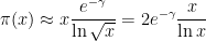
If we repeat for all primes less than or equal to $\sqrt{x}$ , we can conclude that the number of prime numbers less than or equal to $x$ is approximately

$\pi(x) \approx \displaystyle x \prod_{p \le \sqrt{x}} \left(1 - \frac{1}{p} \right)$ .

From this point, we can use Mertens product formula

$\displaystyle \lim_{n \to \infty} \frac{1}{\ln n} \prod_{p \le n} \left(1 - \frac{1}{p} \right)^{-1} = e^\gamma$

to conclude that

$\displaystyle \frac{1}{\ln n} \prod_{p \le n} \left(1 - \frac{1}{p} \right) \approx \displaystyle \frac{e^{-\gamma}}{\ln n}$

if $n$ is large. Therefore,

$\pi(x) \approx x \displaystyle \frac{e^{-\gamma}}{\ln \sqrt{x}} = 2 e^{-\gamma} \displaystyle \frac{x}{\ln x}$ .

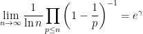
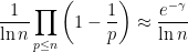
Though not a formal proof, it’s a fast way to convince students that the unusual fraction $\displaystyle \frac{x}{\ln x}$ ought to appear someplace in the prime number theorem.

When I researching for my series of posts on conditional convergence, especially examples related to the constant $\gamma$ , the reference Gamma: Exploring Euler’s Constant by Julian Havil kept popping up. Finally, I decided to splurge for the book, expecting a decent popular account of this number. After all, I’m a professional mathematician, and I took a graduate level class in analytic number theory. In short, I don’t expect to learn a whole lot when reading a popular science book other than perhaps some new pedagogical insights.

Boy, was I wrong. As I turned every page, it seemed I hit a new factoid that I had not known before.

In this series, I’d like to compile some of my favorites — while giving the book a very high recommendation.

What I Learned from Reading “Gamma: Exploring Euler’s Constant” by Julian Havil: Part 16

Let $\pi(n)$ denote the number of positive prime numbers that are less than or equal to $n$ . The prime number theorem, one of the most celebrated results in analytic number theory, states that

$\pi(x) \approx \displaystyle \frac{x}{\ln x}$ .

This is a very difficult result to prove. However, Gamma (page 172) provides a heuristic argument that suggests that this answer might be halfway reasonable.

Consider all of the integers between $1$ and $x$ .

About half of these numbers won’t be divisible by 2.
Of those that aren’t divisible by 2, about two-thirds won’t be divisible by 3. (This isn’t exactly correct, but it’s good enough for heuristics.)
Of those that aren’t divisible by 2 and 3, about four-fifths won’t be divisible by 5.
And so on.

If we repeat for all primes less than or equal to $\sqrt{x}$ , we can conclude that the number of prime numbers less than or equal to $x$ is approximately

$\pi(x) \approx \displaystyle x \prod_{p \le \sqrt{x}} \left(1 - \frac{1}{p} \right)$ .

From this point, we can use Mertens product formula

$\displaystyle \lim_{n \to \infty} \frac{1}{\ln n} \prod_{p \le n} \left(1 - \frac{1}{p} \right)^{-1} = e^\gamma$

to conclude that

$\displaystyle \frac{1}{\ln n} \prod_{p \le n} \left(1 - \frac{1}{p} \right) \approx \displaystyle \frac{e^{-\gamma}}{\ln n}$

if $n$ is large. Therefore,

$\pi(x) \approx x \displaystyle \frac{e^{-\gamma}}{\ln \sqrt{x}} = 2 e^{-\gamma} \displaystyle \frac{x}{\ln x}$ .

Though not a formal proof, it’s a fast way to convince students that the unusual fraction $\displaystyle \frac{x}{\ln x}$ ought to appear someplace in the prime number theorem.

Boy, was I wrong. As I turned every page, it seemed I hit a new factoid that I had not known before.

In this series, I’d like to compile some of my favorites — while giving the book a very high recommendation.

What I Learned from Reading “Gamma: Exploring Euler’s Constant” by Julian Havil: Part 15

I did not know — until I read Gamma (page 168) — that there actually is a formula for generating $n$ th prime number by directly plugging in $n$ . The catch is that it’s a mess:

$p_n = 1 + \displaystyle \sum_{m=1}^{2^n} \left[ n^{1/n} \left( \sum_{i=1}^m \cos^2 \left( \pi \frac{(i-1)!+1}{i} \right) \right)^{-1/n} \right]$ ,

where the outer brackets $[~ ]$ represent the floor function.

This mathematical curiosity has no practical value, as determining the 10th prime number would require computing $1 + 2 + 3 + \dots + 2^{10} = 524,800$ different terms!

Boy, was I wrong. As I turned every page, it seemed I hit a new factoid that I had not known before.

In this series, I’d like to compile some of my favorites — while giving the book a very high recommendation.

What I Learned from Reading “Gamma: Exploring Euler’s Constant” by Julian Havil: Part 14

I hadn’t heard of the worm-on-a-rope problem until I read Gamma (page 133). From Cut-The-Knot:

A worm is at one end of a rubber rope that can be stretched indefinitely. Initially the rope is one kilometer long. The worm crawls along the rope toward the other end at a constant rate of one centimeter per second. At the end of each second the rope is instantly stretched another kilometer. Thus, after the first second the worm has traveled one centimeter, and the length of the rope has become two kilometers. After the second second, the worm has crawled another centimeter and the rope has become three kilometers long, and so on. The stretching is uniform, like the stretching of a rubber band. Only the rope stretches. Units of length and time remain constant.

It turns out that, after $n$ seconds, that the fraction of the band that the worm has traveled is $H_n/N$ , where

$H_n = \displaystyle 1 + \frac{1}{2} + \frac{1}{3} + \dots + \frac{1}{n}$

and $N$ is the length of the rope in centimeters. Using the estimate $H_n \approx \ln n + \gamma$ , we see that the worm will reach the end of the rope when

$H_n = N$

$\ln n + \gamma \approx N$

$\ln n \approx N - \gamma$

$n \approx e^{N - \gamma}$ .

If $N = 100,000$ (since the rope is initially a kilometer long), it will take a really long time for the worm to reach its destination!

Boy, was I wrong. As I turned every page, it seemed I hit a new factoid that I had not known before.

In this series, I’d like to compile some of my favorites — while giving the book a very high recommendation.

What I Learned from Reading “Gamma: Exploring Euler’s Constant” by Julian Havil: Part 13

I hadn’t heard of the crossing-the-desert problem until I read Gamma (page 127). From Wikipedia:

There are n units of fuel stored at a fixed base. The jeep can carry at most 1 unit of fuel at any time, and can travel 1 unit of distance on 1 unit of fuel (the jeep’s fuel consumption is assumed to be constant). At any point in a trip the jeep may leave any amount of fuel that it is carrying at a fuel dump, or may collect any amount of fuel that was left at a fuel dump on a previous trip, as long as its fuel load never exceeds 1 unit…

The jeep must return to the base at the end of every trip except for the final trip, when the jeep travels as far as it can before running out of fuel…

[T]he objective is to maximize the distance traveled by the jeep on its final trip.

The answer is, if $n$ fuel dumps are used, the jeep can go a distance of

$H_n = \displaystyle 1 + \frac{1}{3} + \frac{1}{5} + \dots + \frac{1}{2n-1}$ .

Since the right-hand side approaches infinity as $n$ gets arbitrarily large, it is possible to cross an arbitrarily long desert according the rules of this problem.

Boy, was I wrong. As I turned every page, it seemed I hit a new factoid that I had not known before.

In this series, I’d like to compile some of my favorites — while giving the book a very high recommendation.

What I Learned from Reading “Gamma: Exploring Euler’s Constant” by Julian Havil: Part 12

Let $X_1, X_2, X_3, \dots$ be a sequence of independent and identically distributed random variables, and let $H_n$ be the number of “record highs” upon to and including event $n$ . For example, each $X_i$ can represent the amount of rainfall in a year, where $X_1$ is amount of rainfall recorded the first time that records were kept. As shown in Gamma (page 125), the expected number of record highs is

$H_n = \displaystyle 1 + \frac{1}{2} + \frac{1}{3} + \dots + \frac{1}{n}$ .

As noted in Gamma,

Two arbitrary chosen examples are revealing. The Radcliffe Meteorological Station in Oxford has data for rainfall in Oxford between 1767 and 2000 and there are five record years; this is a span of 234 recorded years and $H_{234} = 6.03$ . For Central Park, New York City, between 1835 and 1994 there are six record years over the 160-year period and $H_{160} = 5.65$ , providing good evidence that English weather is that bit more unpredictable.

Boy, was I wrong. As I turned every page, it seemed I hit a new factoid that I had not known before.

In this series, I’d like to compile some of my favorites — while giving the book a very high recommendation.

What I Learned from Reading “Gamma: Exploring Euler’s Constant” by Julian Havil: Part 11

The Euler-Mascheroni constant $\gamma$ is defined by

$\gamma = \displaystyle \lim_{n \to \infty} \left( \sum_{r=1}^n \frac{1}{r} - \ln n \right)$ .

What I didn’t know, until reading Gamma (page 117), is that there are at least two ways to generalize this definition.

First, $\gamma$ may be thought of as

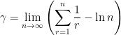$\gamma = \displaystyle \lim_{n \to \infty} \left( \sum_{r=1}^n \frac{1}{\hbox{length of~} [0,r]} - \ln n \right)$ ,

and so this can be generalized to two dimensions as follows:

$\delta = \displaystyle \lim_{n \to \infty} \left( \sum_{r=2}^n \frac{1}{\pi (\rho_r)^2} - \ln n \right)$ ,

where $\rho_r$ is the radius of the smallest disk in the plane containing at least $r$ points $(a,b)$ so that $a$ and $b$ are both integers. This new constant $\delta$ is called the Masser-Gramain constant; like $\gamma$ , the exact value isn’t known.

Second, let $f(x) = \displaystyle \frac{1}{x}$ . Then $\gamma$ may be written as

$\gamma = \displaystyle \lim_{n \to \infty} \left( \sum_{r=1}^n f(r) - \int_1^n f(x) \, dx \right)$ .

Euler (not surprisingly) had the bright idea of changing the function $f(x)$ to any other positive, decreasing function, such as

$f(x) = x^a, \qquad -1 \le a < 0$ ,

producing Euler’s generalized constants. Alternatively (from Stieltjes), we could choose

$f(x) = \displaystyle \frac{ (\ln x)^m }{x}$ .

Boy, was I wrong. As I turned every page, it seemed I hit a new factoid that I had not known before.

In this series, I’d like to compile some of my favorites — while giving the book a very high recommendation.

What I Learned from Reading “Gamma: Exploring Euler’s Constant” by Julian Havil: Part 10

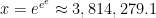
Suppose $p_n$ is the $n$ th prime number, so that $p_{n+1} - p_n$ is the size of the $n$ th gap between successive prime numbers. It turns out (Gamma, page 115) that there’s an incredible theorem for the lower bound of this number:

$\displaystyle \limsup_{n \to \infty} \frac{(p_{n+1}-p_n) (\ln \ln \ln p_n)^2}{(\ln p_n)(\ln \ln p_n)(\ln \ln \ln \ln p_n)} \ge \displaystyle \frac{4 e^{\gamma}}{c}$ ,

where $\gamma$ is the Euler-Mascheroni constant and $c$ is the solution of $c = 3 + e^{-c}$ .

Holy cow, what a formula. Let’s take a look at just a small part of it.

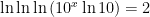
Let’s look at the amazing function $f(x) = \ln \ln \ln \ln x$ , iterating the natural logarithm function four times. This function has a way of converting really large inputs into unimpressive outputs. For example, the canonical “big number” in popular culture is the googolplex, defined as $10^{10^{100}}$ . Well, it takes some work just to rearrange $\displaystyle f \left(10^{10^{100}} \right)$ in a form suitable for plugging into a calculator:

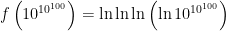
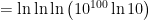
$\displaystyle f \left(10^{10^{100}} \right) = \displaystyle \ln \ln \ln \left( \ln 10^{10^{100}} \right)$

$= \displaystyle \ln \ln \ln \left( 10^{100} \ln 10 \right)$

$= \displaystyle \ln \ln \left[ \ln \left(10^{100} \right) + \ln \ln 10 \right]$

$= \displaystyle \ln \ln \left[ 100 \ln 10 + \ln \ln 10 \right]$

$= \displaystyle \ln \ln \left[ 100 \ln 10 \left( 1 + \frac{\ln \ln 10}{100 \ln 10} \right) \right]$

$= \displaystyle \ln \left( \ln [ 100 \ln 10] + \ln \left( 1 + \frac{\ln \ln 10}{100 \ln 10} \right)\right)$

$\approx 1.6943$

after using a calculator.

This function grows extremely slowly. What value of $x$ gives an output of $0$ ? Well:

$\ln \ln \ln \ln x = 0$

$\ln \ln \ln x = 1$

$\ln \ln x = e$

$\ln x = e^e$

$x = e^{e^e} \approx 3,814,279.1$

What value of $x$ gives an output of $1$ ? Well:

$\ln \ln \ln \ln x = 1$

$\ln \ln \ln x = e$

$\ln \ln x = e^e$

$\ln x = e^{e^e}$

$x = e^{e^{e^e}}$

$\approx e^{3,814,279.1}$

$\approx 10^{3,814,279.1 \log_{10} e}$

$\approx 10^{1,656,420.367636}$

$\approx 2.3315 \times 10^{1,656,420}$

That’s a number with 1,656,421 digits! At the rapid rate of 5 digits per second, it would take over 92 hours (nearly 4 days) just to write out the answer by hand!

Finally, how large does $x$ have to be for the output to be 2? As we’ve already seen, it’s going to be larger than a googolplex:

$\displaystyle f \left(10^{10^{x}} \right) = 2$

$\displaystyle \ln \ln \ln \left( \ln 10^{10^{x}} \right) = 2$

$\displaystyle \ln \ln \ln \left( 10^{x} \ln 10 \right) = 2$

$\displaystyle \ln \ln \left[ \ln \left(10^{x} \right) + \ln \ln 10 \right] = 2$

$\displaystyle \ln \ln \left[ x\ln 10 + \ln \ln 10 \right] = 2$

$\displaystyle \ln \ln \left[ x\ln 10 \left( 1 + \frac{\ln \ln 10}{x\ln 10} \right) \right] = 2$

$\displaystyle \ln \left( \ln [ x\ln 10] + \ln \left( 1 + \frac{\ln \ln 10}{x \ln 10} \right)\right) = 2$

Let’s simplify things slightly by letting $y = x \ln 10$ :

$\displaystyle \ln \left( \ln y + \ln \left( 1 + \frac{\ln \ln 10}{y} \right)\right) = 2$

$\displaystyle \ln y + \ln \left( 1 + \frac{\ln \ln 10}{y} \right) = e^2$

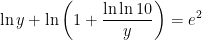
This is a transcendental equation in $y$ ; however, we can estimate that the solution will approximately solve $\ln y = e^2$ since the second term on the left-hand side is small compared to $\ln y$ . This gives the approximation $y = e^{e^2} \approx 1618.18$ . Using either Newton’s method or else graphing the left-hand side yields the more precise solution $y \approx 1617.57$ .

Therefore, $x \approx 1617.57 \ln 10 \approx 3725.99$ , so that

$f \left(10^{10^{3725.99}} \right) \approx 2$ .

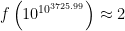One final note: despite what’s typically taught in high school, mathematicians typically use $\log$ to represent natural logarithms (as opposed to base-10 logarithms), so the above formula is more properly written as

$\displaystyle \limsup_{n \to \infty} \frac{(p_{n+1}-p_n) (\log \log \log p_n)^2}{(\log p_n)(\log \log p_n)(\log \log \log \log p_n)} \ge \displaystyle \frac{4 e^{\gamma}}{c}$ .

And this sets up a standard joke, also printed in Gamma:

Q: What noise does a drowning analytic number theorist make?

A: Log… log… log… log…

Boy, was I wrong. As I turned every page, it seemed I hit a new factoid that I had not known before.

In this series, I’d like to compile some of my favorites — while giving the book a very high recommendation.