I'm a Professor of Mathematics and a University Distinguished Teaching Professor at the University of North Texas. For eight years, I was co-director of Teach North Texas, UNT's program for preparing secondary teachers of mathematics and science.
Numerical integration is a standard topic in first-semester calculus. From time to time, I have received questions from students on various aspects of this topic, including:
Why is numerical integration necessary in the first place?
Where do these formulas come from (especially Simpson’s Rule)?
How can I do all of these formulas quickly?
Is there a reason why the Midpoint Rule is better than the Trapezoid Rule?
Is there a reason why both the Midpoint Rule and the Trapezoid Rule converge quadratically?
Is there a reason why Simpson’s Rule converges like the fourth power of the number of subintervals?
In this series, I hope to answer these questions. While these are standard questions in a introductory college course in numerical analysis, and full and rigorous proofs can be found on Wikipedia and Mathworld, I will approach these questions from the point of view of a bright student who is currently enrolled in calculus and hasn’t yet taken real analysis or numerical analysis.
In the previous post in this series, we found that the local error of the left endpoint approximation to was equal to
.
We now consider the global error when integrating over the interval and not just a particular subinterval.
The total error when approximating will be the sum of the errors for the integrals over , , through . Therefore, the total error will be
.
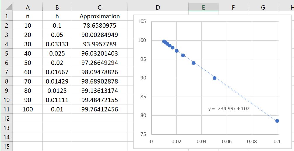
So that this formula doesn’t appear completely mystical, this actually matches the numerical observations that we made earlier. The figure below shows the left-endpoint approximations to for different numbers of subintervals. If we take and , then the error should be approximately equal to
,
which, as expected, is close to the actual error of .
We now perform a more detailed analysis of the global error. Let , so that the error becomes
,
where is the average of the . Clearly, this average is somewhere between the smallest and the largest of the . Since is a continuous function, that means that there must be some value of between and — and therefore between and — so that by the Intermediate Value Theorem. We conclude that the error can be written as
,
Finally, since is the length of one subinterval, we see that is the total length of the interval . Therefore,
,
where the constant is determined by , , and . In other words, for the special case , we have established that the error from the left-endpoint rule is approximately linear in — without resorting to the generalized mean-value theorem.
In my capstone class for future secondary math teachers, I ask my students to come up with ideas for engaging their students with different topics in the secondary mathematics curriculum. In other words, the point of the assignment was not to devise a full-blown lesson plan on this topic. Instead, I asked my students to think about three different ways of getting their students interested in the topic in the first place.
I plan to share some of the best of these ideas on this blog (after asking my students’ permission, of course).
This student submission comes from my former student Brendan Gunnoe. His topic, from Geometry: finding the area of a circle.
History: Squaring the circle
The ancient Greeks and other groups at the time had a fascination with geometry. These cultures tended to like thinking in terms of simpler geometric shapes, such as circles, equilateral triangles and squares. One of the classic problems proposed by these ancient peoples was “Can you create a square with the same area as a circle with finitely many steps only using a compass and straightedge?”. This problem stood for thousands of years, stumping even the most brilliant of mathematicians that attempted to show it true. Eventually, in the year 1882, it was finally proven impossible because of a property of the number π. It’s not too hard to show that π isn’t an integer, nor is it rational. What was left to show is whether π was algebraic or transcendental. The proof from 1882 showed that π is in fact transcendental, proving that it cannot be made using the rules set out by the original question. If a number is algebraic, then it is a solution to a polynomial with rational coefficients.
Curriculum: Using limit of triangular approximations to get the integral
The teacher starts off class by drawing a circle with an inscribed triangle, another with a square, and so on until a hexagon is inscribed. The teacher then draws isosceles triangles that originate at the circles center and extend to the corners of the polygons. The teacher could ask questions like “What do you notice about the total area of the triangles and the area of the circle as we keep adding sides to the polygon?” and “What do you notice about the triangles we made and the little wedges of the circle, what’s the same and what’s different about them?”. Then the teacher could arrange both the triangles and wedges in an alternating up and down fashion, almost like two zippers, to line up the triangles and wedges. The teacher could ask “What’s the length of the top of the triangles? What about the tops of the wedges, what’s their length?”.
Finally, the teacher asks “What happens when we let the number of pieces gets REALLY big? What happens to difference between the area of the triangles and wedges? What about the tops of the triangles and the tops of the wedges?”. In the limit, the upper edge converges to half of the circumference of the circle and the height of the triangles converges to the radius of the circle. Using this line of thinking, the teacher guides the students into seeing how you can derive the equation for the area of a circle by using approximating it with triangles, and then looking at what happens in the limit.
Application
A telescope’s lens is what’s used to control how much light gets into the eye piece. Suppose you’re an astronomer and want to take a photo of the full Moon on a clear night, which gives off 0.25 lumens/s-m2. Suppose your camera needs to get a total of at least 3 lumens to produce a good photo and 5 lumens to get an amazing photo. What’s the radius of a lens (in centimeters) that can take a good photo in 10 minutes? What’s the radius of a lens that can take an amazing photo in 10 minutes?
Now suppose you’re working with the Hubble space telescope in low Earth orbit trying to get photos of a nearby star system. The radius of the main telescope is 120cm and the star system you want to observe is giving off light at a rate of 10-5 lumens/s-m2. How long will it take to get a good photo with Hubble? What about a great photo?
Numerical integration is a standard topic in first-semester calculus. From time to time, I have received questions from students on various aspects of this topic, including:
Why is numerical integration necessary in the first place?
Where do these formulas come from (especially Simpson’s Rule)?
How can I do all of these formulas quickly?
Is there a reason why the Midpoint Rule is better than the Trapezoid Rule?
Is there a reason why both the Midpoint Rule and the Trapezoid Rule converge quadratically?
Is there a reason why Simpson’s Rule converges like the fourth power of the number of subintervals?
In this series, I hope to answer these questions. While these are standard questions in a introductory college course in numerical analysis, and full and rigorous proofs can be found on Wikipedia and Mathworld, I will approach these questions from the point of view of a bright student who is currently enrolled in calculus and hasn’t yet taken real analysis or numerical analysis.
In this post, we will perform an error analysis for the left-endpoint rule
where is the number of subintervals and is the width of each subinterval, so that .
As noted above, a true exploration of error analysis requires the generalized mean-value theorem, which perhaps a bit much for a talented high school student learning about this technique for the first time. That said, the ideas behind the proof are accessible to high school students, using only ideas from the secondary curriculum, if we restrict our attention to the special case , where is a positive integer.
For this special case, the true area under the curve $f(x) = x^k$ on the subinterval will be
In the above, the shorthand can be formally defined, but here we’ll just take it to mean “terms that have a factor of or higher that we’re too lazy to write out.” Since is supposed to be a small number, these terms will be much smaller in magnitude that the terms that have or and thus can be safely ignored.
Using only the left-endpoint of the subinterval, the left-endpoint approximation of is . Therefore, the error in this approximation will be equal to
.
In the next post of this series, we’ll show that the global error when integrating between and — as opposed to between and — is approximately linear in .
In my capstone class for future secondary math teachers, I ask my students to come up with ideas for engaging their students with different topics in the secondary mathematics curriculum. In other words, the point of the assignment was not to devise a full-blown lesson plan on this topic. Instead, I asked my students to think about three different ways of getting their students interested in the topic in the first place.
I plan to share some of the best of these ideas on this blog (after asking my students’ permission, of course).
This student submission again comes from my former student Brendan Gunnoe. His topic: computing the determinant of a matrix.
How can this topic be used in your students’ future courses in mathematics or science?
When students learn about the determinant of a matrix, they only learn about computing it and don’t learn about the applications of the determinant or what they signify. One interesting use of the determinant is finding the eigenvectors of a matrix. A visual understanding of what an eigenvector is can be done by showing what a matrix does to the any generic vector, and what it does to the eigenvectors. For a generic vector that is different from an eigenvector, the matrix knocks the vector off the span of the original vector. What makes an eigenvector special is the fact that the matrix transformation keeps the eigenvector on its span but rescales said eigenvector by its eigenvalue. For example, take the matrix
.
This matrix’s eigenvectors are and with eigenvalues 8 and 2 respectively. That is,
and
.
Eigenvectors have many useful applications in future math and science classes including electronics, linear algebra, differential equations and mechanical engineering.
How can technology (YouTube, Khan Academy [khanacademy.org], Vi Hart, Geometers Sketchpad, graphing calculators, etc.) be used to effectively engage students with this topic? Note: It’s not enough to say “such-and-such is a great website”; you need to explain in some detail why it’s a great website.
The YouTube channel 3Blue1Brown has a fantastic video on determinates and linear transformations. Grant, the channel owner, uses animations to visualize what a matrix transformation does to the plane . He starts by showing what a transformation does to a single square then shows why the change of change of that one area shows what happens to the area of any region. He also gives multiple explanations for what a negative determinate means in terms of orientation of the axes. Then he explains what happens when the determinate is 0. All of this is already extremely useful for understanding what a 2×2 matrix does, but Grant continues and extends all the same things for 3×3 transformations. Lastly, Grant gives a few explanations on why the formula for the determinate is what it is and poses a small puzzle for the viewer to contemplate. This video explains what and why we use determinates and how they can be useful all while showing pleasing visual examples and other explanations.
What interesting word problems using this topic can your students do now?
Using determinates to see if a set of vectors is a basis.
The determinant can tell you when a matrix squishes space into a lower dimensional space like a line or a plane. Thus, taking the determinate of a matrix composed of a set of vectors tells you if those vectors are a basis for the matrix’s dimension.
Part 1. A 3D printer’s axes are set up in such a way that the print head can only travel in the direction and . Assume that the place where the print head is right now is the origin . Can you move the print head to the location and by only moving in the directions of and ?
Hint: Try to solve . Does this always have a solution ?
Part 2. Next time you turn on your 3D printer, one of the motor’s broke and now the print head can only move in the direction of . Assume that the place where the print head is right now is the origin . Can you move the print head to the location by only moving in the direction of ?
Hint: Try to solve . Does this always have a solution ?
Part 3. You buy a new 3D printer that it can move in all three directions: up/down, left/right, forward/backwards. When you test out the movement of the print head, you see that each axis moves in the directions of , , and . Can you use your new 3D printer to go to any location , inside the printing space?
Hint: Think about solving . Does this always have a solution ? How do you know?
Part 4. Your little sibling messed around with your new 3D printer and now it moves in the directions , , and . Is your 3D printer able to get to some point inside the printing space as is, or do you need to fix your printer?
Hint: Think about solving . Does this always have a solution ? How do you know?
Numerical integration is a standard topic in first-semester calculus. From time to time, I have received questions from students on various aspects of this topic, including:
Why is numerical integration necessary in the first place?
Where do these formulas come from (especially Simpson’s Rule)?
How can I do all of these formulas quickly?
Is there a reason why the Midpoint Rule is better than the Trapezoid Rule?
Is there a reason why both the Midpoint Rule and the Trapezoid Rule converge quadratically?
Is there a reason why Simpson’s Rule converges like the fourth power of the number of subintervals?
In this series, I hope to answer these questions. While these are standard questions in a introductory college course in numerical analysis, and full and rigorous proofs can be found on Wikipedia and Mathworld, I will approach these questions from the point of view of a bright student who is currently enrolled in calculus and hasn’t yet taken real analysis or numerical analysis.
In the previous post in this series, I discussed three different ways of numerically approximating the definite integral , the area under a curve between and .
In this series, we’ll choose equal-sized subintervals of the interval . If is the width of each subinterval so that , then the integral may be approximated as
using left endpoints,
using right endpoints, and
using the midpoints of the subintervals. We have also derived the Trapezoid Rule
and Simpson’s Rule (if is even)
.
In the previous post in this series, we saw that both the left-endpoint and right-endpoint rules have a linear rate of convergence: if twice as many subintervals are taken, then the error appears to go down by a factor of 2. If ten times as many subintervals are used, then the error should go down by a factor of 10. However, both the Midpoint Rule and the Trapezoid Rule have a quadratic rate of convergence: if twice as many subintervals are taken, then the error appears to go down by a factor of 4. If ten times as many subintervals are used, then the error should go down by a factor of 100. Moreover, it appears that the error from the Midpoint Rule is about half that of the Trapezoid Rule if the same number of subintervals are used.
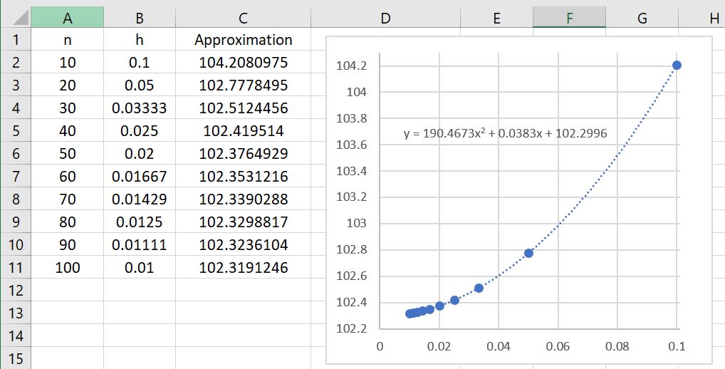
Let’s now explore the results of Simpson’s Rule applied to using different numbers of subintervals. The results are summarized in the table below.
The first immediate observation is that these approximations are far better than even the Midpoint and Trapezoid Rules! Indeed, we see that , using only 20 subintervals, is a better approximation than (from previous posts) either or using 100 subintervals! The lesson to learn again: Simpson’s Rule is a bit more difficult to compute than the Trapezoid Rule or the Midpoint Rule because of the different weights. Nevertheless, choosing a good algorithm is often far better than simply doing lots of computations.
There’s a second observation: the rate of convergence appears to be much, much faster. Indeed, the data points appear to fit a quartic polynomial very well. Said another way, if twice as many subintervals are taken, then the error appears to go down by a factor of 16. We can actually see this in the figure, looking at the lines with 10, 20, 40, and 80 subintervals.
Error with 10 subintervals = .
Error with 20 subintervals = .
Error with 40 subintervals = .
Error with 80 subintervals = .
In all cases, the error on the next line is about the error on the previous line divided by 16.
This illustrates quartic convergence, as opposed to the mere linear convergence of the left- and right-endpoint rules or the quadratic convergence of the Midpoint and Trapezoid Rules.
In my capstone class for future secondary math teachers, I ask my students to come up with ideas for engaging their students with different topics in the secondary mathematics curriculum. In other words, the point of the assignment was not to devise a full-blown lesson plan on this topic. Instead, I asked my students to think about three different ways of getting their students interested in the topic in the first place.
I plan to share some of the best of these ideas on this blog (after asking my students’ permission, of course).
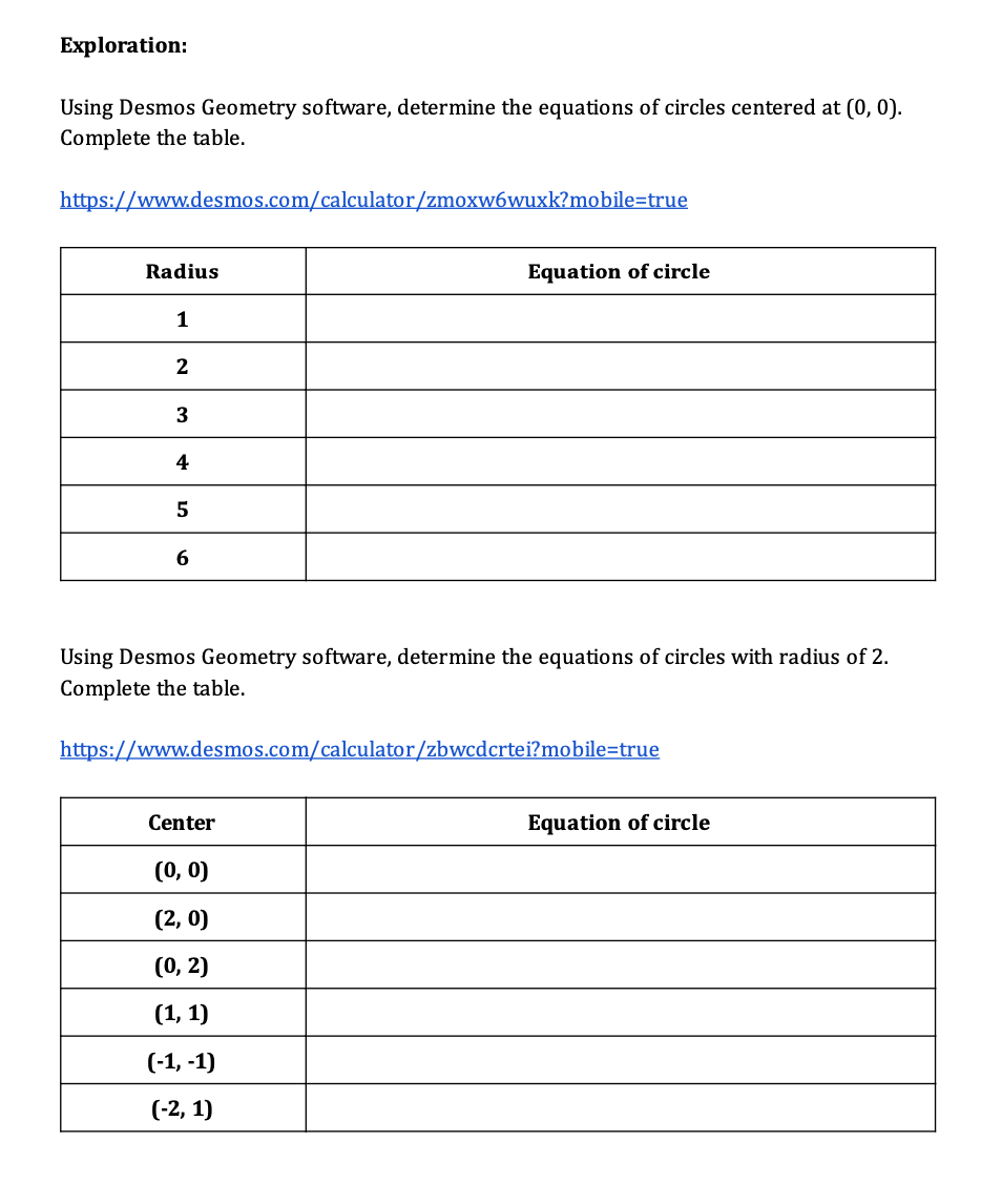
This student submission comes from my former student Noah Mena. His topic, from Precalculus: finding the equation of a circle.
The equation of a circle relies on knowing the definition of a circle, knowing the radius and deciding where the circle is centered at. All of these come into play when a student has to find the equation of a circle. It takes basic understanding of the cartesian grid and understanding the coordinate system. The equation of a circle also builds on students being able to manipulate the equation to get it into standard form and identifying the equation of a circle when it is expanded out. The shape of a circle should also be known, which means with the equation of a circle, students should be able to construct the perfect circle according to the given specifications in the equation.
Learning to write the equation of a circle can be difficult. For one of my teaches last semester my mentor teacher suggested the use of a desmos paired with a worksheet to allow the students to explore what changes the standard equation of a circle. The worksheet had the students enter certain coordinates into the graphing calculator and write down what they thought was the equation of a circle. The next part of the assignment was student driven by having them share their conclusions on what the equation for a circle would be when it is centered at the origin vs. centered at (h,k). The worksheet shows that the students drove their own learning and came to their own conclusions which enhanced engagement through the lesson.
This topic can come up again in trigonometry, upper level calculus and in math modeling. In my TNTX math modeling course, we took a closer look at the derivation of this equation and the subtleties of the standard form. This topic may also be used in physics calculations or in general, science labs. For a physics word problem, it may ask you to calculate the net force and acceleration of a moving object around a circle. In this instance, it would suffice to just know the definition and general shape of a circle to complete these calculations. The definition of a circle is also needed to calculate centripetal force.
Numerical integration is a standard topic in first-semester calculus. From time to time, I have received questions from students on various aspects of this topic, including:
Why is numerical integration necessary in the first place?
Where do these formulas come from (especially Simpson’s Rule)?
How can I do all of these formulas quickly?
Is there a reason why the Midpoint Rule is better than the Trapezoid Rule?
Is there a reason why both the Midpoint Rule and the Trapezoid Rule converge quadratically?
Is there a reason why Simpson’s Rule converges like the fourth power of the number of subintervals?
In this series, I hope to answer these questions. While these are standard questions in a introductory college course in numerical analysis, and full and rigorous proofs can be found on Wikipedia and Mathworld, I will approach these questions from the point of view of a bright student who is currently enrolled in calculus and hasn’t yet taken real analysis or numerical analysis.
In the previous post in this series, I discussed three different ways of numerically approximating the definite integral , the area under a curve between and .
In this series, we’ll choose equal-sized subintervals of the interval . If is the width of each subinterval so that , then the integral may be approximated as
using left endpoints,
using right endpoints, and
using the midpoints of the subintervals. We have also derived the Trapezoid Rule
and Simpson’s Rule (if is even)
.
In the previous post in this series, we saw that both the left-endpoint and right-endpoint rules have a linear rate of convergence: if twice as many subintervals are taken, then the error appears to go down by a factor of 2. If ten times as many subintervals are used, then the error should go down by a factor of 10. However, the Midpoint Rule has a quadratic rate of convergence: if twice as many subintervals are taken, then the error appears to go down by a factor of 4. If ten times as many subintervals are used, then the error should go down by a factor of 100.
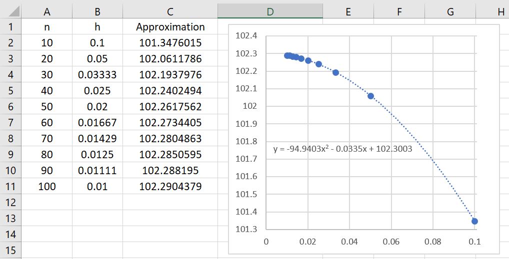
Let’s now explore the results of the Trapezoid Rule applied to using different numbers of subintervals. The results are summarized in the table below.
Once again, the data points fit a quadratic polynomial well, indicating quadratic convergence.
More subtly, it appears that the Trapezoid Rule isn’t quite as good as the Midpoint Rule. Here are the results from the Midpoint Rule (which also appeared in the previous post in this series):
For subintervals, the error of the Trapezoid Rule is , which the error from the Midpoint Rule is . In other words, while both of these methods are superior to the left- and right-endpoint rules, it appears that the error from the Midpoint Rule is about half of the error from the Trapezoid Rule. The Midpoint Rule appears to be better.
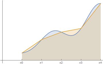
To me, this is far from an obvious conclusion. Geometrically, it’s far from clear that the rectangles from the Midpoint Rule…
… provide a better approximation than using trapezoids …
… yet it appears that’s exactly what happened. This can be rigorously proven, as we’ll explore later in this series.
In my capstone class for future secondary math teachers, I ask my students to come up with ideas for engaging their students with different topics in the secondary mathematics curriculum. In other words, the point of the assignment was not to devise a full-blown lesson plan on this topic. Instead, I asked my students to think about three different ways of getting their students interested in the topic in the first place.
I plan to share some of the best of these ideas on this blog (after asking my students’ permission, of course).
This student submission comes from my former student Austin Stone. His topic, from Precalculus: solving exponential equations.
What interesting (i.e., uncontrived) word problems using this topic can your students do now?
Exponential equations can be used in lots of different kinds of word problems. One that is pretty common but is very useful for students involves interest rate. “Megan has $20,000 to invest for 5 years and she found an interest rate of 5%. How much money will she have at the end of 5 years if the interest rate compounds monthly?” I would give them the formula A=P(1+r/n)rt. It is pretty easy to convince students that this is a real-world problem and would get the students engaged about exponential equations. You can also reword the problem to ask for how much Megan started with, what the rate is, or how much time the money was in there. That way students get used to solving equations when the variable is in the exponent and when it is not. This also can lead into or us prior knowledge of natural log to solve for the variable in the exponent.
How could you as a teacher create an activity or project that involves your topic?
Using the basis of the problem I mentioned above, a teacher could create a Project Based Instruction lesson using this idea. The teacher can set up a scenario where, over the course of a week or two, the students would have to decide which bank to make an investment in by calculating how much money they would profit at each bank. The students would have to research different banks and their interest rate. The teacher could also give each group different scenarios where some groups have more money to invest. Students would have to figure out how long they would like to invest. The teacher would give Do It Yourselves and Workshops that deal with solving exponential equations and also getting used to natural log. They would then make a presentation explaining what bank they have chosen and why. They would also have to explain the math that they would have used.
How has this topic appeared in the news?
To say that exponential equations have been in the news lately would be an understatement. It has virtually been the news this year. COVID-19 is a virus and viruses spread exponentially. This would get students engaged immediately because the topic would be relatable to their own lives. Doctors and scientists try to figure out different ways to “flatten the curve”, which essentially means to make the spread of the virus not exponential anymore. We have all heard people on the news telling the public how to stop the virus from spreading and how not make people around you at risk of contracting it (contributing the exponential spread). We all have most likely seen a doctor or scientist show a graph of the virus’s spread and their predictions on how it will look in the upcoming weeks. This would give students a chance to see that what they are learning can be applied to very crucial things going on in the world around them.
Numerical integration is a standard topic in first-semester calculus. From time to time, I have received questions from students on various aspects of this topic, including:
Why is numerical integration necessary in the first place?
Where do these formulas come from (especially Simpson’s Rule)?
How can I do all of these formulas quickly?
Is there a reason why the Midpoint Rule is better than the Trapezoid Rule?
Is there a reason why both the Midpoint Rule and the Trapezoid Rule converge quadratically?
Is there a reason why Simpson’s Rule converges like the fourth power of the number of subintervals?
In this series, I hope to answer these questions. While these are standard questions in a introductory college course in numerical analysis, and full and rigorous proofs can be found on Wikipedia and Mathworld, I will approach these questions from the point of view of a bright student who is currently enrolled in calculus and hasn’t yet taken real analysis or numerical analysis.
In the previous post in this series, I discussed three different ways of numerically approximating the definite integral , the area under a curve between and .
In this series, we’ll choose equal-sized subintervals of the interval . If is the width of each subinterval so that , then the integral may be approximated as
using left endpoints,
using right endpoints, and
using the midpoints of the subintervals. We have also derived the Trapezoid Rule
and Simpson’s Rule (if is even)
.
In the previous post in this series, we saw that both the left-endpoint and right-endpoint rules have a linear rate of convergence: if twice as many subintervals are taken, then the error appears to go down by a factor of 2. If ten times as many subintervals are used, then the error should go down by a factor of 10. Let’s now explore the results of the midpoint rule applied to using different numbers of subintervals. The results are summarized in the table below. The first immediate observation is that these approximations are far better than the left- and right-endpoint rule approximations! Indeed, we see that , using only ten subintervals, is a far better approximation than (from the previous post) either or using 100 subintervals! The lesson to learn: choosing a good algorithm is often far better than simply doing lots of computations.
There’s a second observation: the rate of convergence appears to be much, much faster. Indeed, the data points appear to fit a parabola very well instead of a straight line. Said another way, if twice as many subintervals are taken, then the error appears to go down by a factor of 4. If ten times as many subintervals are used, then the error should go down by a factor of 100. This illustrates quadratic convergence, as opposed to the mere linear convergence of the left- and right-endpoint rules.
In my capstone class for future secondary math teachers, I ask my students to come up with ideas for engaging their students with different topics in the secondary mathematics curriculum. In other words, the point of the assignment was not to devise a full-blown lesson plan on this topic. Instead, I asked my students to think about three different ways of getting their students interested in the topic in the first place.
I plan to share some of the best of these ideas on this blog (after asking my students’ permission, of course).
This student submission comes from my former student Mason Maynard. His topic, from Precalculus: compound interest.
What interesting (i.e., uncontrived) word problems using this topic can your students do now? (You may find resources such as http://www.spacemath.nasa.gov to be very helpful in this regard; feel free to suggest others.)
A deposit of $3000 earns 2% interest compounded semiannually. How much money is in the bank after for 4 years?
A deposit of $2150 earns 6% interest compounded quarterly. How much money is in the bank after for 6 years?
A deposit of $495 earns 3% interest compounded annually. How much money is in the bank after for 3 years?
These word problems are some of the basic compound interest problems that your students learn how to do where you just plug in the correct values for their corresponding variables.
If you invested $1,000 in an account paying an annual percentage rate (quoted rate) compounded daily (based on a bank year of 360 days) and you wanted to have $2,500 in your account at the end of your investment time, what interest rate would you need if the investment time were 1 year, 10 years, 20 years, 100 years?
If you invested $500 in an account paying an annual percentage rate compounded quarterly , and you wanted to have $2,500 in your account at the end of your investment time, what interest rate would you need if the investment time were 1 year, 10 years, 20 years, 100 years?
These are the types of problems that get more difficult for the students. You want them to use compound interest to solve but then they must incorporate logs into their solutions because they are looking for time instead of interest.
How does this topic extend what your students should have learned in previous courses?
With compound interest, students first learn about the simple interest formula. The only main difference is that you start to include exponents with compound interests. Then when you introduce your students to compound interest, you start to get into some more complicated problems. After they learn about compound interest and its basic problems, then you transition into logs with your students. This is used in compound interest and instead of just looking for the interest that will be accumulated after a specific amount of time, you then shift the variable around that you are looking for. The most coming type of problem that refers to this is they give you all of the information except for the amount time it takes to get a certain amount of interest. The last thing that leads up to compound interest in Calculus is when you transition from calculating the amount of interested over specific time intervals and a specific amount of times you compound it to calculating it with compounding it continuously over a specific time interval.
How have different cultures throughout time used this topic in their society?
Interest is something you have to pay on a load. Depending on what side you are and how thinks go, you are either getting some more money back that what you invested or you are paying off a massive debt. Some think that the idea behind charging loans on interest came from the early days of neighbors loaning there cattle to one another. What is really unique about this is that the words in the Egyptian, ancient Greek and Sumerian languages is connected to cattle and their offspring. This leads some to believe that interest came about due to the natural increase of the herd that occurred when you loaned out your cattle.
The first evidence that comes of a compound interest problem dates back to 2000-1700 B.C. in Babylon. A clay tablet was found and the unique thing is that the interest rate use to solve it was not written. Some researchers assume that the rate was 20% due to that mainly all the other compound interest problems dating back closer to this used it. What is really crazy is that 20% worked to solve the problem. The only thing that was wrong was that the time was corresponding to the Babylon calendar of 360 days instead of our 365 days.
In 50 B.C. Cicero writes to a friend in Rome. The letter tells that he would not normally recognize more than 12 percent interest on a loan, even though a decree was passed which required money lenders to charge no more than 12 percent. Cicero would then write a few days later that they will pay back the loan in 6 years will 12 percent interest and more money will be added each year.

 was equal to

![[a,b]](https://s0.wp.com/latex.php?latex=%5Ba%2Cb%5D&bg=ffffff&fg=000000&s=0&c=20201002) and not just a particular subinterval.
and not just a particular subinterval. will be the sum of the errors for the integrals over
 ![[x_0,x_1]](https://s0.wp.com/latex.php?latex=%5Bx_0%2Cx_1%5D&bg=ffffff&fg=000000&s=0&c=20201002) ,
, ![[x_1,x_2]](https://s0.wp.com/latex.php?latex=%5Bx_1%2Cx_2%5D&bg=ffffff&fg=000000&s=0&c=20201002) , through
, through ![[x_{n-1},x_n]](https://s0.wp.com/latex.php?latex=%5Bx_%7Bn-1%7D%2Cx_n%5D&bg=ffffff&fg=000000&s=0&c=20201002) . Therefore, the total error will be
. Therefore, the total error will be

 for different numbers of subintervals. If we take
  and
and  , then the error should be approximately equal to

 .
.
 , so that the error becomes

 is the average of the
  . Clearly, this average is somewhere between the smallest and the largest of the
  is a continuous function, that means that there must be some value of
  between
  and
and  — and therefore between
  and
and  — so that
  by the Intermediate Value Theorem. We conclude that the error can be written as

 is the length of one subinterval, we see that
  is the total length of the interval
 is determined by
  . In other words, for the special case
  , we have established that the error from the left-endpoint rule is approximately linear in
 ![\int_a^b f(x) \, dx \approx h \left[f(x_0) + f(x_1) + \dots + f(x_{n-1}) \right] \equiv L_n](https://s0.wp.com/latex.php?latex=%5Cint_a%5Eb+f%28x%29+%5C%2C+dx+%5Capprox+h+%5Cleft%5Bf%28x_0%29+%2B+f%28x_1%29+%2B+%5Cdots+%2B+f%28x_%7Bn-1%7D%29+%5Cright%5D+%5Cequiv+L_n&bg=ffffff&fg=000000&s=0&c=20201002)
 is the number of subintervals and
  is the width of each subinterval, so that
  .
.
 is a positive integer.
![[x_i, x_i +h]](https://s0.wp.com/latex.php?latex=%5Bx_i%2C+x_i+%2Bh%5D&bg=ffffff&fg=000000&s=0&c=20201002) will be
will be![\displaystyle \int_{x_i}^{x_i+h} x^k \, dx = \frac{1}{k+1} \left[ (x_i+h)^{k+1} - x_i^{k+1} \right]](https://s0.wp.com/latex.php?latex=%5Cdisplaystyle+%5Cint_%7Bx_i%7D%5E%7Bx_i%2Bh%7D+x%5Ek+%5C%2C+dx+%3D+%5Cfrac%7B1%7D%7Bk%2B1%7D+%5Cleft%5B+%28x_i%2Bh%29%5E%7Bk%2B1%7D+-+x_i%5E%7Bk%2B1%7D+%5Cright%5D&bg=ffffff&fg=000000&s=0&c=20201002)
![= \displaystyle \frac{1}{k+1} \left[x_i^{k+1} + {k+1 \choose 1} x_i^k h + {k+1 \choose 2} x_i^{k-1} h^2 + O(h^3) - x_i^{k+1} \right]](https://s0.wp.com/latex.php?latex=%3D+%5Cdisplaystyle+%5Cfrac%7B1%7D%7Bk%2B1%7D+%5Cleft%5Bx_i%5E%7Bk%2B1%7D+%2B+%7Bk%2B1+%5Cchoose+1%7D+x_i%5Ek+h+%2B+%7Bk%2B1+%5Cchoose+2%7D+x_i%5E%7Bk-1%7D+h%5E2+%2B+O%28h%5E3%29+-+x_i%5E%7Bk%2B1%7D+%5Cright%5D&bg=ffffff&fg=000000&s=0&c=20201002)
![= \displaystyle \frac{1}{k+1} \left[ (k+1) x_i^k h + \frac{(k+1)k}{2} x_i^{k-1} h^2 + O(h^3) \right]](https://s0.wp.com/latex.php?latex=%3D+%5Cdisplaystyle+%5Cfrac%7B1%7D%7Bk%2B1%7D+%5Cleft%5B+%28k%2B1%29+x_i%5Ek+h+%2B+%5Cfrac%7B%28k%2B1%29k%7D%7B2%7D+x_i%5E%7Bk-1%7D+h%5E2+%2B+O%28h%5E3%29+%5Cright%5D&bg=ffffff&fg=000000&s=0&c=20201002)

 can be formally defined, but here we’ll just take it to mean “terms that have a factor of
  or higher that we’re too lazy to write out.” Since
  and thus can be safely ignored.
 . Therefore, the error in this approximation will be equal to
 and
and  — is approximately linear in
 ![\left[ \begin{array}{cc} 5 & 3 \\ 3 & 5 \end{array} \right]](https://s0.wp.com/latex.php?latex=%5Cleft%5B+%5Cbegin%7Barray%7D%7Bcc%7D+5+%26+3+%5C%5C+3+%26+5+%5Cend%7Barray%7D+%5Cright%5D&bg=ffffff&fg=000000&s=0&c=20201002) .
.![\left[ \begin{array}{c} 1 \\ 1 \end{array} \right]](https://s0.wp.com/latex.php?latex=%5Cleft%5B+%5Cbegin%7Barray%7D%7Bc%7D+1+%5C%5C+1+%5Cend%7Barray%7D+%5Cright%5D&bg=ffffff&fg=000000&s=0&c=20201002) and
and ![\left[ \begin{array}{c} 1 \\ -1 \end{array} \right]](https://s0.wp.com/latex.php?latex=%5Cleft%5B+%5Cbegin%7Barray%7D%7Bc%7D+1+%5C%5C+-1+%5Cend%7Barray%7D+%5Cright%5D&bg=ffffff&fg=000000&s=0&c=20201002) with eigenvalues 8 and 2 respectively. That is,
with eigenvalues 8 and 2 respectively. That is,![\left[ \begin{array}{cc} 5 & 3 \\ 3 & 5 \end{array} \right] \left[ \begin{array}{c} 1 \\ 1 \end{array} \right] = \left[ \begin{array}{c} 8 \\ 8 \end{array} \right] = 8 \left[ \begin{array}{c} 1 \\ 1 \end{array} \right]](https://s0.wp.com/latex.php?latex=%5Cleft%5B+%5Cbegin%7Barray%7D%7Bcc%7D+5+%26+3+%5C%5C+3+%26+5+%5Cend%7Barray%7D+%5Cright%5D+%5Cleft%5B+%5Cbegin%7Barray%7D%7Bc%7D+1+%5C%5C+1+%5Cend%7Barray%7D+%5Cright%5D+%3D+%5Cleft%5B+%5Cbegin%7Barray%7D%7Bc%7D+8+%5C%5C+8+%5Cend%7Barray%7D+%5Cright%5D+%3D%26nbsp%3B8+%5Cleft%5B+%5Cbegin%7Barray%7D%7Bc%7D+1+%5C%5C+1+%5Cend%7Barray%7D+%5Cright%5D&bg=ffffff&fg=000000&s=0&c=20201002)
![\left[ \begin{array}{cc} 5 & 3 \\ 3 & 5 \end{array} \right] \left[ \begin{array}{c} 1 \\ -1 \end{array} \right] = \left[ \begin{array}{c} 2 \\ -2 \end{array} \right] = 2 \left[ \begin{array}{c} 1 \\ -1 \end{array} \right]](https://s0.wp.com/latex.php?latex=%5Cleft%5B+%5Cbegin%7Barray%7D%7Bcc%7D+5+%26+3+%5C%5C+3+%26+5+%5Cend%7Barray%7D+%5Cright%5D+%5Cleft%5B+%5Cbegin%7Barray%7D%7Bc%7D+1+%5C%5C+-1+%5Cend%7Barray%7D+%5Cright%5D+%3D+%5Cleft%5B+%5Cbegin%7Barray%7D%7Bc%7D+2+%5C%5C+-2+%5Cend%7Barray%7D+%5Cright%5D+%3D+2+%5Cleft%5B+%5Cbegin%7Barray%7D%7Bc%7D+1+%5C%5C+-1+%5Cend%7Barray%7D+%5Cright%5D&bg=ffffff&fg=000000&s=0&c=20201002) .
.![\left[ \begin{array}{c} -1 \\ 1 \end{array} \right]](https://s0.wp.com/latex.php?latex=%5Cleft%5B+%5Cbegin%7Barray%7D%7Bc%7D+-1+%5C%5C+1+%5Cend%7Barray%7D+%5Cright%5D&bg=ffffff&fg=000000&s=0&c=20201002) . Assume that the place where the print head is right now is the origin
. Assume that the place where the print head is right now is the origin ![\left[ \begin{array}{c} 0 \\ 0 \end{array} \right]](https://s0.wp.com/latex.php?latex=%5Cleft%5B+%5Cbegin%7Barray%7D%7Bc%7D+0+%5C%5C+0+%5Cend%7Barray%7D+%5Cright%5D&bg=ffffff&fg=000000&s=0&c=20201002) . Can you move the print head to the location
. Can you move the print head to the location ![\left[ \begin{array}{c} x \\ y \end{array} \right]](https://s0.wp.com/latex.php?latex=%5Cleft%5B+%5Cbegin%7Barray%7D%7Bc%7D+x+%5C%5C+y+%5Cend%7Barray%7D+%5Cright%5D&bg=ffffff&fg=000000&s=0&c=20201002) and
and ![\left[ \begin{array}{cc} 1 & -1 \\ 1 & 1 \end{array} \right] \left[ \begin{array}{c} a \\ b \end{array} \right] = \left[ \begin{array}{c} x \\ y \end{array} \right]](https://s0.wp.com/latex.php?latex=%5Cleft%5B+%5Cbegin%7Barray%7D%7Bcc%7D+1+%26+-1+%5C%5C+1+%26+1+%5Cend%7Barray%7D+%5Cright%5D+%5Cleft%5B+%5Cbegin%7Barray%7D%7Bc%7D+a+%5C%5C+b+%5Cend%7Barray%7D+%5Cright%5D+%3D+%5Cleft%5B+%5Cbegin%7Barray%7D%7Bc%7D+x+%5C%5C+y+%5Cend%7Barray%7D+%5Cright%5D&bg=ffffff&fg=000000&s=0&c=20201002) . Does this always have a solution
. Does this always have a solution ![\left[ \begin{array}{c} a \\ b \end{array} \right]](https://s0.wp.com/latex.php?latex=%5Cleft%5B+%5Cbegin%7Barray%7D%7Bc%7D+a+%5C%5C+b+%5Cend%7Barray%7D+%5Cright%5D&bg=ffffff&fg=000000&s=0&c=20201002) ?
?![\left[ \begin{array}{c} 1 \\ 0 \end{array} \right]](https://s0.wp.com/latex.php?latex=%5Cleft%5B+%5Cbegin%7Barray%7D%7Bc%7D+1+%5C%5C+0+%5Cend%7Barray%7D+%5Cright%5D&bg=ffffff&fg=000000&s=0&c=20201002) . Assume that the place where the print head is right now is the origin
. Assume that the place where the print head is right now is the origin ![\left[ \begin{array}{cc} 1 & 0 \\ 0 & 0 \end{array} \right] \left[ \begin{array}{c} a \\ b \end{array} \right] = \left[ \begin{array}{c} x \\ y \end{array} \right]](https://s0.wp.com/latex.php?latex=%5Cleft%5B+%5Cbegin%7Barray%7D%7Bcc%7D+1+%26+0+%5C%5C+0+%26+0+%5Cend%7Barray%7D+%5Cright%5D+%5Cleft%5B+%5Cbegin%7Barray%7D%7Bc%7D+a+%5C%5C+b+%5Cend%7Barray%7D+%5Cright%5D+%3D+%5Cleft%5B+%5Cbegin%7Barray%7D%7Bc%7D+x+%5C%5C+y+%5Cend%7Barray%7D+%5Cright%5D&bg=ffffff&fg=000000&s=0&c=20201002) . Does this always have a solution
. Does this always have a solution ![\left[ \begin{array}{c} 1 \\ 0 \\ 0 \end{array} \right]](https://s0.wp.com/latex.php?latex=%5Cleft%5B+%5Cbegin%7Barray%7D%7Bc%7D+1+%5C%5C+0+%5C%5C+0+%5Cend%7Barray%7D+%5Cright%5D&bg=ffffff&fg=000000&s=0&c=20201002) ,
, ![\left[ \begin{array}{c} 0 \\ 1 \\ 0 \end{array} \right]](https://s0.wp.com/latex.php?latex=%5Cleft%5B+%5Cbegin%7Barray%7D%7Bc%7D+0+%5C%5C+1+%5C%5C+0+%5Cend%7Barray%7D+%5Cright%5D&bg=ffffff&fg=000000&s=0&c=20201002) , and
, and ![\left[ \begin{array}{c} 0 \\ 0 \\ 1 \end{array} \right]](https://s0.wp.com/latex.php?latex=%5Cleft%5B+%5Cbegin%7Barray%7D%7Bc%7D+0+%5C%5C+0+%5C%5C+1+%5Cend%7Barray%7D+%5Cright%5D&bg=ffffff&fg=000000&s=0&c=20201002) . Can you use your new 3D printer to go to any location
. Can you use your new 3D printer to go to any location ![\left[ \begin{array}{c} x \\ y \\ z \end{array} \right]](https://s0.wp.com/latex.php?latex=%5Cleft%5B+%5Cbegin%7Barray%7D%7Bc%7D+x+%5C%5C+y+%5C%5C+z+%5Cend%7Barray%7D+%5Cright%5D&bg=ffffff&fg=000000&s=0&c=20201002) , inside the printing space?
, inside the printing space?![\left[ \begin{array}{ccc} 1 & 0 & 0 \\ 0 & 1 & 0 \\ 0 & 0 & 1 \end{array} \right] \left[ \begin{array}{c} a \\ b \\ c \end{array} \right] = \left[ \begin{array}{c} x \\ y \\ z \end{array} \right]](https://s0.wp.com/latex.php?latex=%5Cleft%5B+%5Cbegin%7Barray%7D%7Bccc%7D+1+%26+0+%26+0+%5C%5C+0+%26+1+%26+0+%5C%5C+0+%26+0+%26+1+%5Cend%7Barray%7D+%5Cright%5D+%5Cleft%5B+%5Cbegin%7Barray%7D%7Bc%7D+a+%5C%5C+b+%5C%5C+c+%5Cend%7Barray%7D+%5Cright%5D+%3D+%5Cleft%5B+%5Cbegin%7Barray%7D%7Bc%7D+x+%5C%5C+y+%5C%5C+z+%5Cend%7Barray%7D+%5Cright%5D&bg=ffffff&fg=000000&s=0&c=20201002) . Does this always have a solution
. Does this always have a solution ![\left[ \begin{array}{c} a \\ b \\ c \end{array} \right]](https://s0.wp.com/latex.php?latex=%5Cleft%5B+%5Cbegin%7Barray%7D%7Bc%7D+a+%5C%5C+b+%5C%5C+c+%5Cend%7Barray%7D+%5Cright%5D&bg=ffffff&fg=000000&s=0&c=20201002) ? How do you know?
? How do you know?![\left[ \begin{array}{c} 1 \\ 0 \\ 1 \end{array} \right]](https://s0.wp.com/latex.php?latex=%5Cleft%5B+%5Cbegin%7Barray%7D%7Bc%7D+1+%5C%5C+0+%5C%5C+1+%5Cend%7Barray%7D+%5Cright%5D&bg=ffffff&fg=000000&s=0&c=20201002) ,
, ![\left[ \begin{array}{c} 1 \\ 1 \\ 0 \end{array} \right]](https://s0.wp.com/latex.php?latex=%5Cleft%5B+%5Cbegin%7Barray%7D%7Bc%7D+1+%5C%5C+1+%5C%5C+0+%5Cend%7Barray%7D+%5Cright%5D&bg=ffffff&fg=000000&s=0&c=20201002) , and
, and ![\left[ \begin{array}{c} 2 \\ 1 \\ 1 \end{array} \right]](https://s0.wp.com/latex.php?latex=%5Cleft%5B+%5Cbegin%7Barray%7D%7Bc%7D+2+%5C%5C+1+%5C%5C+1+%5Cend%7Barray%7D+%5Cright%5D&bg=ffffff&fg=000000&s=0&c=20201002) . Is your 3D printer able to get to some point
. Is your 3D printer able to get to some point ![\left[ \begin{array}{ccc} 1 & 1 & 2 \\ 0 & 1 & 1 \\ 1 & 0 & 1 \end{array} \right] \left[ \begin{array}{c} a \\ b \\ c \end{array} \right] = \left[ \begin{array}{c} x \\ y \\ z \end{array} \right]](https://s0.wp.com/latex.php?latex=%5Cleft%5B+%5Cbegin%7Barray%7D%7Bccc%7D+1+%26+1+%26+2+%5C%5C+0+%26+1+%26+1+%5C%5C+1+%26+0+%26+1+%5Cend%7Barray%7D+%5Cright%5D+%5Cleft%5B+%5Cbegin%7Barray%7D%7Bc%7D+a+%5C%5C+b+%5C%5C+c+%5Cend%7Barray%7D+%5Cright%5D+%3D+%5Cleft%5B+%5Cbegin%7Barray%7D%7Bc%7D+x+%5C%5C+y+%5C%5C+z+%5Cend%7Barray%7D+%5Cright%5D&bg=ffffff&fg=000000&s=0&c=20201002) . Does this always have a solution
. Does this always have a solution  , the area under a curve
  between
  and
and  .
.
![\int_a^b f(x) \, dx \approx h \left[f(x_1) + f(x_2) + \dots + f(x_n) \right] \equiv R_n](https://s0.wp.com/latex.php?latex=%5Cint_a%5Eb+f%28x%29+%5C%2C+dx+%5Capprox+h+%5Cleft%5Bf%28x_1%29+%2B+f%28x_2%29+%2B+%5Cdots+%2B+f%28x_n%29+%5Cright%5D+%5Cequiv+R_n&bg=ffffff&fg=000000&s=0&c=20201002)
![\int_a^b f(x) \, dx \approx h \left[f(c_1) + f(c_2) + \dots + f(c_n) \right] \equiv M_n](https://s0.wp.com/latex.php?latex=%5Cint_a%5Eb+f%28x%29+%5C%2C+dx+%5Capprox+h+%5Cleft%5Bf%28c_1%29+%2B+f%28c_2%29+%2B+%5Cdots+%2B+f%28c_n%29+%5Cright%5D+%5Cequiv+M_n&bg=ffffff&fg=000000&s=0&c=20201002)
![\int_a^b f(x) \, dx \approx \displaystyle \frac{h}{2} [f(x_0) + 2f(x_1) + \dots + 2f(x_{n-1}) + f(x_n)] \equiv T_n](https://s0.wp.com/latex.php?latex=%5Cint_a%5Eb+f%28x%29+%5C%2C+dx+%5Capprox+%5Cdisplaystyle+%5Cfrac%7Bh%7D%7B2%7D+%5Bf%28x_0%29+%2B+2f%28x_1%29+%2B+%5Cdots+%2B+2f%28x_%7Bn-1%7D%29+%2B+f%28x_n%29%5D+%5Cequiv+T_n&bg=ffffff&fg=000000&s=0&c=20201002)
![\int_a^b f(x) \, dx \approx \displaystyle \frac{h}{3} \left[y_0 + 4 y_1 + 2 y_2 + 4 y_3 + \dots + 2y_{n-2} + 4 y_{n-1} + y_{n} \right] \equiv S_n](https://s0.wp.com/latex.php?latex=%5Cint_a%5Eb+f%28x%29+%5C%2C+dx+%5Capprox+%5Cdisplaystyle+%5Cfrac%7Bh%7D%7B3%7D+%5Cleft%5By_0+%2B+4+y_1+%2B+2+y_2+%2B+4+y_3+%2B+%5Cdots+%2B+2y_%7Bn-2%7D+%2B+4+y_%7Bn-1%7D+%2B%C2%A0+y_%7Bn%7D+%5Cright%5D+%5Cequiv+S_n&bg=ffffff&fg=000000&s=0&c=20201002) .
. using different numbers of subintervals. The results are summarized in the table below.
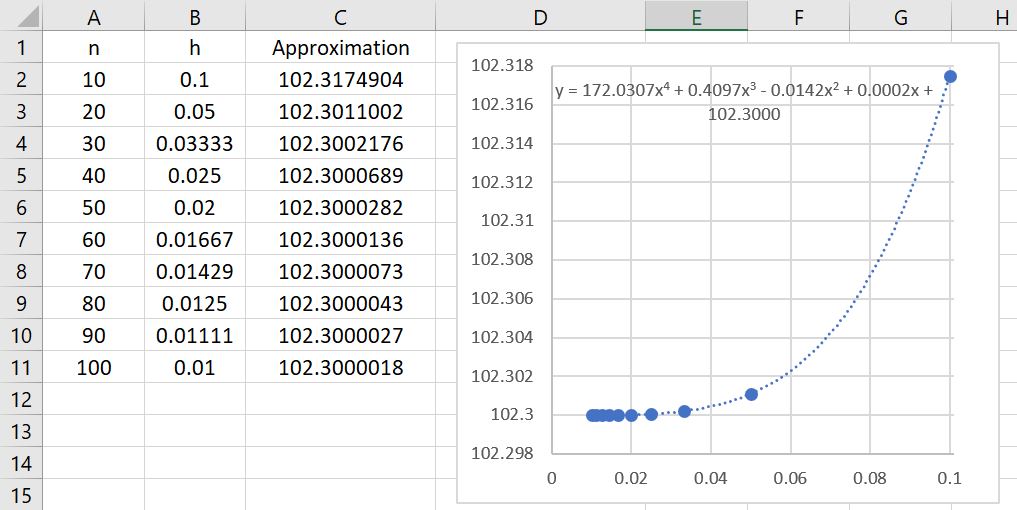
 , using only 20 subintervals, is a better approximation than (from previous posts) either
  or
or  using 100 subintervals! The lesson to learn again: Simpson’s Rule is a bit more difficult to compute than the Trapezoid Rule or the Midpoint Rule because of the different weights. Nevertheless, choosing a good algorithm is often far better than simply doing lots of computations.
  .
. .
. .
. .
.
 , which the error from the Midpoint Rule is
  . In other words, while both of these methods are superior to the left- and right-endpoint rules, it appears that the error from the Midpoint Rule is about half of the error from the Trapezoid Rule. The Midpoint Rule appears to be better.
 , using only ten subintervals, is a far better approximation than (from the previous post) either
  or
or  using 100 subintervals! The lesson to learn: choosing a good algorithm is often far better than simply doing lots of computations.