Interdisciplinary studies (Part 4)

Shamelessly stolen from a friend:

How do you tell the difference between a plumber and a chemist?

Ask them to pronounce unionized.

Continued fractions and pi

I suggest the following activity for bright middle-school students who think that they know everything that there is to know about fractions.

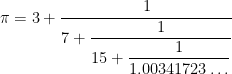
The approximation to $\pi$ that is most commonly taught to students is $\displaystyle \frac{22}{7}$ . As I’ll discuss, this is the closest rational number to $\pi$ using a denominator less than $100$ . However, it is possible to obtain closer rational approximations to $\pi$ using larger numbers. Indeed, the ancient Chinese mathematicians were superior to the ancient Greeks in this regard, as they developed the approximation

$\pi \approx \displaystyle \frac{355}{133}$

It turns out that this is the best rational approximation to $\pi$ using a denominator less than $16,000$ . In other words, $\displaystyle \frac{355}{133}$ is the best approximation to $\pi$ using a reasonably simple rational number.

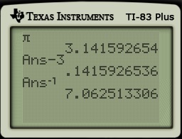
Step 1. To begin, let’s find $\pi$ with a calculator. Then let’s now subtract $3$ and then find the inverse.

This calculation has shown that

$\pi = \displaystyle 3 + \frac{1}{7.0625133\dots}$

If we ignore the $0.0625133$ , we obtain the usual approximation

$\pi \approx \displaystyle 3 + \frac{1}{7} = \frac{22}{7}$

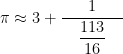
Step 2. However, there’s no reason to stop with one reciprocal, and this might give us some even better approximations. Let’s subtract $7$ from the current denominator and find the reciprocal of the difference.

At this point, we have shown that

$\pi = \displaystyle 3 + \frac{1}{7 + \displaystyle\frac{1}{15.9965944\dots}}$

If we round the final denominator down to $15$ , we obtain the approximation

$\pi \approx \displaystyle 3 + \frac{1}{7 + \displaystyle\frac{1}{15}}$

$\pi \approx \displaystyle 3 + \frac{1}{~~~\displaystyle \frac{106}{15}~~~}$

$\pi \approx \displaystyle 3 + \frac{15}{106}$

$\pi \approx \displaystyle \frac{333}{106}$

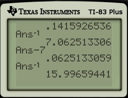
Step 3. Continuing with the next denominator, we subtract $15$ and take the reciprocal again.

At this point, we have shown that

$\pi = \displaystyle 3 + \frac{1}{7 + \displaystyle\frac{1}{15 + \displaystyle \frac{1}{1.00341723\dots}}}$

If we round the final denominator down to $1$ , we obtain the approximation

$\pi \approx \displaystyle 3 + \frac{1}{7 + \displaystyle\frac{1}{16}}$

$\pi \approx \displaystyle 3 + \frac{1}{~~~\displaystyle \frac{113}{16}~~~}$

$\pi \approx \displaystyle 3 + \frac{16}{113}$

$\pi \approx \displaystyle \frac{355}{113}$

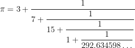
Step 4. Let me show one more step.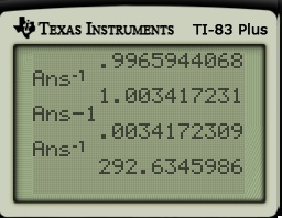

At this point, we have shown that

$\pi = \displaystyle 3 + \frac{1}{7 + \displaystyle\frac{1}{15 + \displaystyle \frac{1}{1 + \displaystyle \frac{1}{292.634598\dots}}}}$

If we round the final denominator down to $292$ , we (eventually) obtain the approximation

$\pi \approx \displaystyle \frac{52163}{16604}$

The calculations above are the initial steps in finding the continued fraction representation of $\pi$ . A full treatment of continued fractions is well outside the scope of a single blog post. Instead, I’ll refer the interested reader to the good write-ups at MathWorld (http://mathworld.wolfram.com/ContinuedFraction.html) and Wikipedia (http://en.wikipedia.org/wiki/Continued_fraction) as well as the references therein.

But I would like to point out one important property of the convergents that we found above, which were

$\displaystyle \frac{22}{7}, \frac{333}{106}, \frac{355}{113}, ~ \hbox{and} ~ \frac{52163}{16604}$

All of these fractions are pretty close to $\pi$ , as shown below. (The first decimal below is the result for $22/7$ .)

In fact, these are the first terms in a sequence of best possible rational approximations to $\pi$ up to the given denominator. In other words:

$\displaystyle \frac{22}{7}$ is the best rational approximation to $\pi$ using a denominator less than $106$. In other words, no integer over $8$ will be any closer to $\pi$ than $\displaystyle \frac{22}{7}$ . No integer over $9$ will be any closer to $\pi$ than $\displaystyle \frac{22}{7}$ . And so on, all the way up to denominators of $105$ . Small wonder that we usually teach children the approximation $\pi \approx \displaystyle \frac{22}{7}$ .
Once we reach $106$ , the fraction $\displaystyle \frac{323}{106}$ is the best rational approximation to $\pi$ using a denominator less than $113$ .
Then $\displaystyle \frac{355}{113}$ is the best rational approximation to $\pi$ using a denominator less than $16604$ .

As noted above, the ancient Chinese mathematicians were superior to the ancient Greeks in this regard, as they were able to develop the approximation $\pi \approx \displaystyle \frac{355}{113}$ . For example, Archimedes was able to establish that

$3\frac{10}{71} < \pi < 3\frac{1}{7}$

Engaging students: The field axioms

In my capstone class for future secondary math teachers, I ask my students to come up with ideas for engaging their students with different topics in the secondary mathematics curriculum. In other words, the point of the assignment was not to devise a full-blown lesson plan on this topic. Instead, I asked my students to think about three different ways of getting their students interested in the topic in the first place.

I plan to share some of the best of these ideas on this blog (after asking my students’ permission, of course).

This student submission again comes from my former student Maranda Edmonson. Her topic, from Pre-Algebra: the field axioms of arithmetic (the distributive law, the commutativity and associativity of addition and multiplication, etc.).

B. Curriculum: How can this topic be used in your students’ future courses in mathematics or science?

It is safe to say that the field axioms are used in all mathematics classes once they are introduced. As students, we know them to be rules for how to simplify or expand expressions, solving equations, or just manipulating numbers and expressions. As instructors, we know them to be a solid foundation for further mathematical understanding. “In mathematics or logic, [an axiom is] an unprovable rule or first principle accepted to be true because it is self-evident or particularly useful” (Merriam-Webster.com). Is the distributive property not useful? Isn’t the associative property self-evident? We learn these axioms, master them during the first lesson we encounter them, and they stick with us. Why? Because they are obvious “rules” that we use and apply to all aspects of mathematics. They are a foundation on which we, as instructors, wish to build upon a greater mathematical understanding.

B. Curriculum: How does this idea extend what your students should have learned in previous courses?

When students first begin to learn addition they are learning the associative property as well. Think about it – when kids learn about the expanded form of a number, they are already seeing that when you add more than two numbers together they equal the same thing, no matter what order they are being added in. For example:

$1,458 = 1,000 + 400 + 50 + 8 = (1,000 + 400) + (50 + 8) = (1,000 + 50) + (400 + 8)$

and so on. Kids tend to add numbers in the order that they are given. However, when they start learning little tricks (say, their tens facts), then they will start seeing how the numbers work together. For example: $3 + 4 + 7$ soon becomes $(3 + 7) + 4$ . Then, when students get into higher grades and begin learning multiplication, the commutative property becomes a real focus. When they are learning their multiplication facts, students are faced with $5 \times 7$ one minute, then $7 \times 5$ the next. They start seeing that it does not matter what order the numbers are in, but that when two numbers are being multiplied together, they will equal the same product each time.

E. Technology: How can technology be used to effectively engage students with this topic?

Math and music are always a good combination. Honestly, who doesn’t hum “Pop! Goes the Weasel” every time they need to use the quadratic formula? This YouTube video (the link is below) is of some students singing a song about the associative, commutative and distributive properties. The video is difficult to hear unless you turn the volume up, and the quality is not the greatest. However, the students in the video get the point across about what the axioms are and that they only apply to addition and multiplication. Note that you only need to watch the first three minutes of the video. The last minute and a half or so is irrelevant to the axioms themselves.

Full lesson plan: Designing a model solar system

Over the summer, I occasionally teach a small summer math class for my daughter and her friends around my dining room table. Mostly to preserve the memory for future years… and to provide a resource to my friends who wonder what their children are learning… I’ll write up the best of these lesson plans in full detail.

This was a fun activity that took a couple of hours: designing a model Solar System. I chose the scale so that most of the planets would fit on a straight section of sidewalk near my house; of course, the scale could be changed to fit the available space.

For my particular audience of students, I also worked through the basics of the metric system as well as decimals.

This lesson plan is written in a 5E format — engage, explore, explain, elaborate, evaluate — which promotes inquiry-based learning and fosters student engagement.

Model Solar System Handout

Model Solar System Lesson

Post Assessment

P.S. For what it’s worth, the world’s largest model solar system can be found in Sweden.

Engaging students: Order of operations

I plan to share some of the best of these ideas on this blog (after asking my students’ permission, of course).

This student submission comes from my former student Alyssa Dalling. Her topic, from Pre-Algebra: order of operations.

C. How has this topic appeared in pop culture (movies, TV, current music, video games, etc.)?

Hannah Montana is a Disney series that aired from 2006-2011. On this episode titled “Sleepwalk This Way”, Miley’s dad writes her a new song which she reads and doesn’t like. She decides to keep her dislike of the new song to herself causing her to start sleepwalking. In order to not tell her dad what she thinks of the song while sleepwalking, Miley stops sleeping which causes her many problems. One such problem occurs when Miley gets dressed in the wrong order causing her to get an unwanted result.

I would start out the class by showing the first 46 seconds of this Hannah Montana scene. (Editor’s note: Trust me, this is hilarious.) This scene is perfect for the engage because it is a way to relate the order of operations to getting dressed. After watching the scene, the teacher would explain that just like getting dressed in the proper order is important, the order of operations when doing math is as well. The students would learn PEMDAS (parenthesis, exponents, multiplication, division, addition, and subtraction) and try different problems to get them better acquainted with the concept.

B. How can this topic be used in your students’ future courses in mathematics or science?

The order of operations will be used in almost every math class following Pre-Algebra. One example is in Algebra II when students start working with problems involving simplifying numbers and multiple variables. One example is

$\left( \displaystyle \frac{18a^{4x} b^2}{-6 a^x b^5} \right)^3$

Start out the class by asking students how the order of operations says to answer this question. Most students will follow method two below. Upon completion of this lesson, students will learn multiple methods of problem solving which expand their previous knowledge of order of operations.

The first method students can use is to raise the numerator and denominator to the third power before simplifying. By raising each variable to the third power, no rules in the order of operations will be broken showing the student there is more than one way to use the order of operations. (Reference Method One below).

The method most students will originally think of is simplifying the fraction before raising it to the third power. The student would follow their previous knowledge of PEMDAS in order to simplify the equation to the reduced form. (Reference Method Two below). In either case, the students will see that the solution can be found by using a variety of different means that all fall under the order of operations.

Method One:

Method Two:

Resources: http://www.glencoe.com/sec/math/algebra/algebra2/algebra2_05/extra_examples/chapter5/lesson5_1.pdf

B. How can this topic be used in your students’ future courses in mathematics or science?

An understanding of the order of operations is relied upon in Calculus as well. One application is when learning the chain rule. The following YouTube video does a fun job at explaining the chain rule by using a catchy song. The students are able to learn the rule and see examples that they can use to help them with this concept. Start it at 1:32 and end it at 2:10 (shown below).

The chain rule is used to find the derivative of the composition of two functions. So if $f$ and $g$ are functions, then the derivative of $f(g(x))$ can be found using the chain rule. Using the example $F(x) = (x^3+5x)^2$ , the chain rule states that the derivative will be $F'(x) = f'(z) g'(x)$ . Following this definition, the student finds the derivative to be $2(x^3+5x)(3x^2+5)$ . This is where the order of operations comes in. The student must use their previously acquired skills from Pre-Algebra as well as Algebra II to simplify the expression. From their previously acquired knowledge, the student would know they would have to multiply the $2$ by each expression in $f'(z)$ . Also, if a question asked the student to find the derivative when $x=3$ , the student would have to use their knowledge of the order of operations to find the solution after applying the chain rule.

Resources: http://archives.math.utk.edu/visual.calculus/2/chain_rule.4/index.html

Engaging students: Finding x- and y-intercepts

I plan to share some of the best of these ideas on this blog (after asking my students’ permission, of course).

This student submission again comes from my former student Maranda Edmonson. Her topic, from Algebra: finding $x-$ and $y-$ intercepts. Unlike most student submissions, Maranda’s idea answers three different questions at once.

Applications: How could you as a teacher create an activity or project that involves your topic?

Culture: How has this topic appeared in pop culture (movies, TV, current music, video games, etc.)?

Technology: How can technology be used to effectively engage students with this topic?

This link is to a reflection by a mathematics teacher who used the popular TV show “The Big Bang Theory” to teach linear functions. She taught this lesson prior to teaching students about finding $y-$ intercepts of linear functions, but it can be adapted in order to teach how to find the intercepts themselves.

ENGAGE:

One thing I would not change would be to show the students the above clip of the show where Howard and Sheldon are heatedly discussing crickets at the beginning of the activity. By showing the video at the beginning, students will be engaged and want to figure out what will be done throughout the lesson. Being a clip of a popular show that many probably watch during the week, students will be even more engaged and interested since they are able to watch something that they are already familiar with. Being something that they are already familiar with or can relate to, students have a tendency to remember the material or at least the topic longer than they would remember something that they were unfamiliar with or could not relate.

In the clip, Sheldon argues that the cricket the guys hear while eating dinner is a snowy tree cricket based on the temperature of the room and the frequency of chirps; Howard argues that it is an ordinary field cricket. The beginning of their discussion is as follows:

Sheldon: “Based on the number of chirps per minute, and the ambient temperature in this room, it is a snowy tree cricket.”

Howard: “Oh, give me a frickin’ break. How could you possibly know that?”

Sheldon: “In 1890, Amos Dolbear determined that there was a fixed relationship between the number of chirps per minute of the snowy tree cricket and the ambient temperature – a precise relationship that is not present with ordinary field crickets.”

The whole episode revolves around the guys finding the exact genus and species of the cricket, but that is not the importance here. The importance of this clip is the linear relationship between the temperature and the number of chirps per minute of the cricket, which the activity should then be centered around.

EXPLORE:

After showing the short clip, it could be beneficial to show students the Wikipedia link that discusses Dolbear’s Law. Toward the bottom of the page, the relationship is written out in several formats, but there is a basic linear function that students could focus on for the activity.

Assuming students know how to graph linear functions (as stated above, the link is for a lesson the teacher taught before teaching students about $y-$ intercepts), I would have students graph Dolbear’s Law on a piece of graph paper. The challenge would be for students to find out what happens when there are variations to the number of chirps of the cricket, the temperature or both to see how the graph changes – specifically where the graph crosses each axis.

EXPLAIN/ELABORATE/EVALUATE:

At this point, students should be able to state what changes they noticed with the graph – specifically where the graph crossed the axes as changes are made to the function. After they have explained what they found, fill in any gaps and correct vocabulary as needed. Basically, teach what little there is left for the lesson. Follow-up by providing extra examples or a worksheet for students to practice before giving them a quiz or test to assess their performance.

E=mc2

Source: https://www.facebook.com/photo.php?fbid=546898598706809&set=a.261051580624847.62913.133949023335104&type=1&theater

Non-geometric infinite series (Part 12)

I conclude this series of posts with thoughts about infinite series which use reciprocals of positive integers. I offer this post for the enrichment of talented Precalculus students who have exhibited mastery of geometric series.

Geometric. As we’ve discussed at length, the series

$1 + \displaystyle \frac{1}{2} + \frac{1}{4} + \frac{1}{8} + \frac{1}{16} + \dots$

converges and is in fact equal to $2$ .

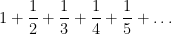
Harmonic. Including the reciprocals of all positive integers is called a harmonic series:

$1 + \displaystyle \frac{1}{2} + \frac{1}{3} + \frac{1}{4} + \frac{1}{5} + \dots$

As shown in the link to the MathWorld website, this series actually diverges, even though the terms get smaller and smaller.

So we’ve made an observation: if too many reciprocals are included, the series diverges. But if we take enough of them away, then we can still end up with a series that is infinite but converges.

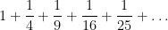
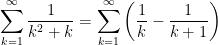
Squares. Let’s now consider the reciprocals of perfect squares:

$1 + \displaystyle \frac{1}{4} + \frac{1}{9} + \frac{1}{16} + \frac{1}{25} + \dots$

Clearly, we’ve taken away a lot of the terms of the harmonic series? Have we taken enough away so that the series converges? It turns out that the answer is yes. And the answer is precisely what you’d think it should be (not): $\pi^2/6$ . This is just another way that the circumference of a circle has an odd way of appearing in the most unexpected of places.

The proof that this series equals $\pi^2/6$ requires the clever use of Parseval’s theorem from Fourier analysis.

Fourth Powers. Let’s now turn to the reciprocals of fourth powers:

$1 + \displaystyle \frac{1}{16} + \frac{1}{81} + \frac{1}{256} + \frac{1}{625} + \dots$

By the Direct Comparison Test and the series for reciprocals of squares, this series converges. Using Parseval’s theorem, it can be shown that the answer is $\pi^4/90$ .

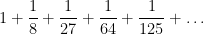
Cubes. Now let’s investigate the reciprocals of cubes:

$1 + \displaystyle \frac{1}{8} + \frac{1}{27} + \frac{1}{64} + \frac{1}{125} + \dots$

Again by the Direct Comparison Test and the series for reciprocals for squares, this series must converge. This sum is called Apéry’s constant. However, and amazingly, no one knows what the answer is. Of course, a computer can be programmed to evaluate this series to as many decimal places as desired. According to Wikipedia, this sum was evaluated to over 100 billion decimal places in 2010. However, to the best of my knowledge, no one has figured out if there’s a simple way of writing the answer, like $\pi^2/6$ or $\pi^4/90$ .

So if you figure out a simple way to evaluate Apéry’s constant, feel free to call me collect.

The previous four series are example of Riemann’s zeta function, which is of central importance in number theory and is the focus of the celebrated Riemann Hypothesis, for which a solution is worth a cool $1 million.

Primes. Now let’s consider the reciprocals of primes:

$\displaystyle \frac{1}{2} + \frac{1}{3} + \frac{1}{5} + \frac{1}{7} + \frac{1}{11} + \dots$

As noted above, the harmonic series diverges, but if we remove enough terms from the harmonic series, then it’s possible to make an infinite series that converges. So the central question is, did we remove enough fractions (by taking away all of the composite denominators) so that the series converges?

Surprisingly, the answer is no: the sum of the reciprocals of the primes actually diverges. The proof actually requires a graduate-level class in analytic number theory.

By no means would I expect high school students to master all of the above facts. As noted above, the subject of this post is mostly for the enrichment of high school students who have mastered infinite geometric series.

That said, students who know the following facts from Precalculus will be well-served when they reach calculus and other university-level mathematics courses.

They should either know the formula for an infinite geometric series or else be able to quickly derive it.
They should know that not every infinite geometric series is geometric.
They should know that not every infinite series converges.
They should be familiar with the meaning of the terms converge and diverge.

Formula for an infinite geometric series (Part 11)

Many math majors don’t have immediate recall of the formula for an infinite geometric series. They often can remember that there is a formula, but they can’t recollect the details. While it’s I think it’s OK that they don’t have the formula memorized, I think is a real shame that they’re also unaware of where the formula comes from and hence are unable to rederive the formula if they’ve forgotten it.

In this post, I’d like to give some thoughts about why the formula for an infinite geometric series is important for other areas of mathematics besides Precalculus. (There may be others, but here’s what I can think of in one sitting.)

1. An infinite geometric series is actually a special case of a Taylor series. (See https://meangreenmath.com/2013/07/05/reminding-students-about-taylor-series-part-5/ for details.) Therefore, it would be wonderful if students learning Taylor series in Calculus II could be able to relate the new topic (Taylor series) to their previous knowledge (infinite geometric series) which they had already seen in Precalculus.

2. An infinite geometric series is also a special case of the binomial series $(1+x)^n$ , when $n$ does not have to be a positive integer and hence Pascal’s triangle cannot be used to find the expansion.

3. Infinite geometric series is a rare case when an infinite sum can be found exactly. In Calculus II, a whole battery of tests (e.g., the Root Test, the Ratio Test, the Limit Comparison Test) are introduced to determine whether a series converges or not. In other words, these tests only determine if an answer exists, without determining what the answer actually is.

Throughout the entire undergraduate curriculum, I’m aware of only four types of series that can actually be evaluated exactly.

An infinite geometric series with $-1 < r < 1$
The Taylor series of a real analytic function. (Of course, an infinite geometric series is a special case of a Taylor series.)
A telescoping series. For example, using partial fractions and cancelling a bunch of terms, we find that

$\displaystyle \sum_{k=1}^\infty \frac{1}{k^2+k} = \displaystyle \sum_{k=1}^\infty \left( \frac{1}{k} - \frac{1}{k+1} \right)$

$\displaystyle \sum_{k=1}^\infty \frac{1}{k^2+k} = \displaystyle \left( 1 - \frac{1}{2} \right) + \left( \frac{1}{2} - \frac{1}{3} \right) \dots$

$\displaystyle \sum_{k=1}^\infty \frac{1}{k^2+k} = 1$

An infinite series that arises from Parseval’s theorem in Fourier analysis.

4. Infinite geometric series are essential for proving basic facts about decimal representations that we often take for granted.

We can justify why $0.\overline{9} = 1$ . See https://meangreenmath.com/2013/09/03/why-does-0-999-1-part-3/ for details.
Along with the Direct Comparison Test, we can be used to justify why a decimal representation $0.d_1d_2d_3\dots$ actually converges and must correspond to a real number. See https://meangreenmath.com/2013/09/01/why-does-0-999-1-part-1/ for details.
We can prove that a fraction of the form $\displaystyle \frac{M}{10^k-1}$ must have a repeating block of length $k$ which contains the digits of $M$ . See https://meangreenmath.com/2013/08/22/thoughts-on-17-and-other-rational-numbers-part-5/ for details.
Going the other direction, we can also convert an repeating decimal representation into a fraction. See https://meangreenmath.com/2013/08/21/thoughts-on-17-and-other-rational-numbers-part-4/ for details.
We can also find representations in other bases besides base 10. See https://meangreenmath.com/2013/08/17/calculator-errors-when-close-isnt-close-enough-part-2 for an example of a repeating binary representation.

5. Properties of an infinite geometric series are needed to find the mean and standard deviation of a geometric random variable, which is used to predict the number of independent trials needed before an event happens. This is used for analyzing the coupon collector’s problem, among other applications.

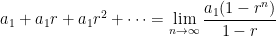
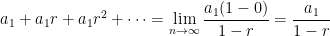
Formula for an infinite geometric series (Part 10)

I conclude this series of posts by considering the formula for an infinite geometric series. Somewhat surprisingly (to students), the formula for an infinite geometric series is actually easier to remember than the formula for a finite geometric series.

One way of deriving the formula parallels the derivation for a finite geometric series. If $a_1, a_2, a_3, \dots$ are the first terms of an infinite geometric sequence, let

$S = a_1 + a_2 + a_3 + \dots$

Recalling the formula for an geometric sequence, we know that

$a_2 = a_1 r$

$a_3 = a_1 r^2$

$\vdots$

Substituting, we find

$S = a_1 + a_1 r+ a_1 r^2 \dots$

Once again, we multiply both sides by $-r$ .

$-rS = -a_1r - a_1 r^2- a_1 r^3 \dots$

Next, we add the two equations. Notice that almost everything cancels on the right-hand side… except for the leading term $a_1$ . (Unlike yesterday’s post, there is no “last” term that remains since the series is infinite.) Therefore,

$S - rS = a_1$

$S(1-r) = a_1$

$S = \displaystyle \frac{a_1}{1-r}$

A quick pedagogical note: I find that this derivation “sells” best to students when I multiply by $-r$ and add, as opposed to multiplying by $r$ and subtracting.

The above derivation is helpful for remembering the formula but glosses over an extremely important detail: not every infinite geometric series converges. For example, if $a_1 = 1$ and $r = 2$ , then the infinite geometric series becomes

$1 + 2 + 4 + 8 + 16 + \dots$ ,

which clearly does not have a finite answer. We say that this series diverges. In other words, trying to evaluate this sum makes as much sense as trying to divide a number by zero: there is no answer.

That said, it can be shown that, as long as $-1 < r < 1$ , then the above geometric series converges, so that

$a_1 + a_1 r + a_1 r^2 + \dots = \displaystyle \frac{a_1}{1-r}$

The formal proof requires the use of the formula for a finite geometric series:

$a_1 + a_1 r + a_1 r^2 + \dots + a_1 r^{n-1} = \displaystyle \frac{a_1(1-r^n)}{1-r}$

We then take the limit as $n \to \infty$ :

$\displaystyle \lim_{n \to \infty} a_1 + a_1 r + a_1 r^2 + \dots + a_1 r^{n-1} = \displaystyle \lim_{n \to \infty} \frac{a_1(1-r^n)}{1-r}$

$a_1 + a_1 r + a_1 r^2 + \dots = \displaystyle \lim_{n \to \infty} \frac{a_1(1-r^n)}{1-r}$

On the right-hand side, the only piece that contains an $n$ is the term $r^n$ . If $-1 < r < 1$ , then $r^n \to 0$ as $n \to \infty$ . (This limit fails, however, if $r \ge 1$ or $r \le -1$ .) Therefore,