My Favorite One-Liners: Part 35

In this series, I’m compiling some of the quips and one-liners that I’ll use with my students to hopefully make my lessons more memorable for them.

Every once in a while, I’ll discuss something in class which is at least tangentially related to an unsolved problems in mathematics. For example, when discussing infinite series, I’ll ask my students to debate whether or not this series converges:

$1 + \frac{1}{10} + \frac{1}{100} + \frac{1}{1000} + \dots$

Of course, this one converges since it’s an infinite geometric series. Then we’ll move on to an infinite series that is not geometric:

$1 + \frac{1}{4} + \frac{1}{9} + \frac{1}{16} + \dots$ ,

where the denominators are all perfect squares. I’ll have my students guess about whether or not this one converges. It turns out that it does, and the answer is exactly what my students should expect the answer to be, $\pi^2/6$ .

Then I tell my students, that was a joke (usually to relieved laughter).

Next, I’ll put up the series

$1 + \frac{1}{8} + \frac{1}{27} + \frac{1}{64} + \dots$ ,

where the denominators are all perfect cubes. I’ll have my students guess about whether or not this one converges. Usually someone will see that this one has to converge since the previous one converged and the terms of this one are pairwise smaller than the previous series — an intuitive use of the Dominated Convergence Test. Then, I’ll ask, what does this converge to?

The answer is, nobody knows. It can be calculated to very high precision with modern computers, of course, but it’s unknown whether there’s a simple expression for this sum.

So, concluding the story whenever I present an unsolved problem, I’ll tell my students,

If you figure out the answer, call me, and call me collect.

What I Learned from Reading “Gamma: Exploring Euler’s Constant” by Julian Havil: Part 13

I hadn’t heard of the crossing-the-desert problem until I read Gamma (page 127). From Wikipedia:

There are n units of fuel stored at a fixed base. The jeep can carry at most 1 unit of fuel at any time, and can travel 1 unit of distance on 1 unit of fuel (the jeep’s fuel consumption is assumed to be constant). At any point in a trip the jeep may leave any amount of fuel that it is carrying at a fuel dump, or may collect any amount of fuel that was left at a fuel dump on a previous trip, as long as its fuel load never exceeds 1 unit…

The jeep must return to the base at the end of every trip except for the final trip, when the jeep travels as far as it can before running out of fuel…

[T]he objective is to maximize the distance traveled by the jeep on its final trip.

The answer is, if $n$ fuel dumps are used, the jeep can go a distance of

$H_n = \displaystyle 1 + \frac{1}{3} + \frac{1}{5} + \dots + \frac{1}{2n-1}$ .

Since the right-hand side approaches infinity as $n$ gets arbitrarily large, it is possible to cross an arbitrarily long desert according the rules of this problem.

When I researching for my series of posts on conditional convergence, especially examples related to the constant $\gamma$ , the reference Gamma: Exploring Euler’s Constant by Julian Havil kept popping up. Finally, I decided to splurge for the book, expecting a decent popular account of this number. After all, I’m a professional mathematician, and I took a graduate level class in analytic number theory. In short, I don’t expect to learn a whole lot when reading a popular science book other than perhaps some new pedagogical insights.

Boy, was I wrong. As I turned every page, it seemed I hit a new factoid that I had not known before.

In this series, I’d like to compile some of my favorites — while giving the book a very high recommendation.

Thoughts on Infinity: Index

I’m doing something that I should have done a long time ago: collect past series of posts into a single, easy-to-reference post. The following posts formed my series on various lessons I’ve learned while trying to answer the questions posed by gifted elementary school students.

Part 1: Different types of countable sets

Part 2a: Divergence of the harmonic series.

Part 2b: Convergence of the Kempner series.

Part 3a: Conditional convergent series or products shouldn’t be rearranged.

Part 3b: Definition of the Euler-Mascheroni constant $\gamma$ .

Part 3c: Evaluation of the conditionally convergent series $\displaystyle 1 - \frac{1}{2} + \frac{1}{3} - \frac{1}{4} + \frac{1}{5} \dots$

Part 3d: Confirmation of this evaluation using technology.

Part 3e: Evaluation of a rearrangement of this conditionally convergent series.

Part 3f: Confirmation of this different evaluation using technology.

Part 3g: Closing thoughts.

Reminding students about Taylor series (Part 4)

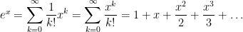
I’m in the middle of a series of posts describing how I remind students about Taylor series. In the previous posts, I described how I lead students to the definition of the Maclaurin series

$f(x) = \displaystyle \sum_{k=0}^{\infty} \frac{f^{(k)}(0)}{k!} x^k$ ,

which converges to $f(x)$ within some radius of convergence for all functions that commonly appear in the secondary mathematics curriculum.

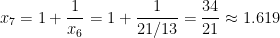
Step 4. Let’s now get some practice with Maclaurin series. Let’s start with $f(x) = e^x$ .

What’s $f(0)$ ? That’s easy: $f(0) = e^0 = 1$ .

Next, to find $f'(0)$ , we first find $f'(x)$ . What is it? Well, that’s also easy: $f'(x) = \frac{d}{dx} (e^x) = e^x$ . So $f'(0)$ is also equal to $1$ .

How about $f''(0)$ ? Yep, it’s also $1$ . In fact, it’s clear that $f^{(n)}(0) = 1$ for all $n$ , though we’ll skip the formal proof by induction.

Plugging into the above formula, we find that

$e^x = \displaystyle \sum_{k=0}^{\infty} \frac{1}{k!} x^k = \sum_{k=0}^{\infty} \frac{x^k}{k!} = 1 + x + \frac{x^2}{2} + \frac{x^3}{3} + \dots$

It turns out that the radius of convergence for this power series is $\infty$ . In other words, the series on the right converges for all values of $x$ . So we’ll skip this for review purposes, this can be formally checked by using the Ratio Test.

At this point, students generally feel confident about the mechanics of finding a Taylor series expansion, and that’s a good thing. However, in my experience, their command of Taylor series is still somewhat artificial. They can go through the motions of taking derivatives and finding the Taylor series, but this complicated symbol in $\displaystyle \sum$ notation still doesn’t have much meaning.

So I shift gears somewhat to discuss the rate of convergence. My hope is to deepen students’ knowledge by getting them to believe that $f(x)$ really can be approximated to high precision with only a few terms. Perhaps not surprisingly, it converges quicker for small values of $x$ than for big values of $x$ .

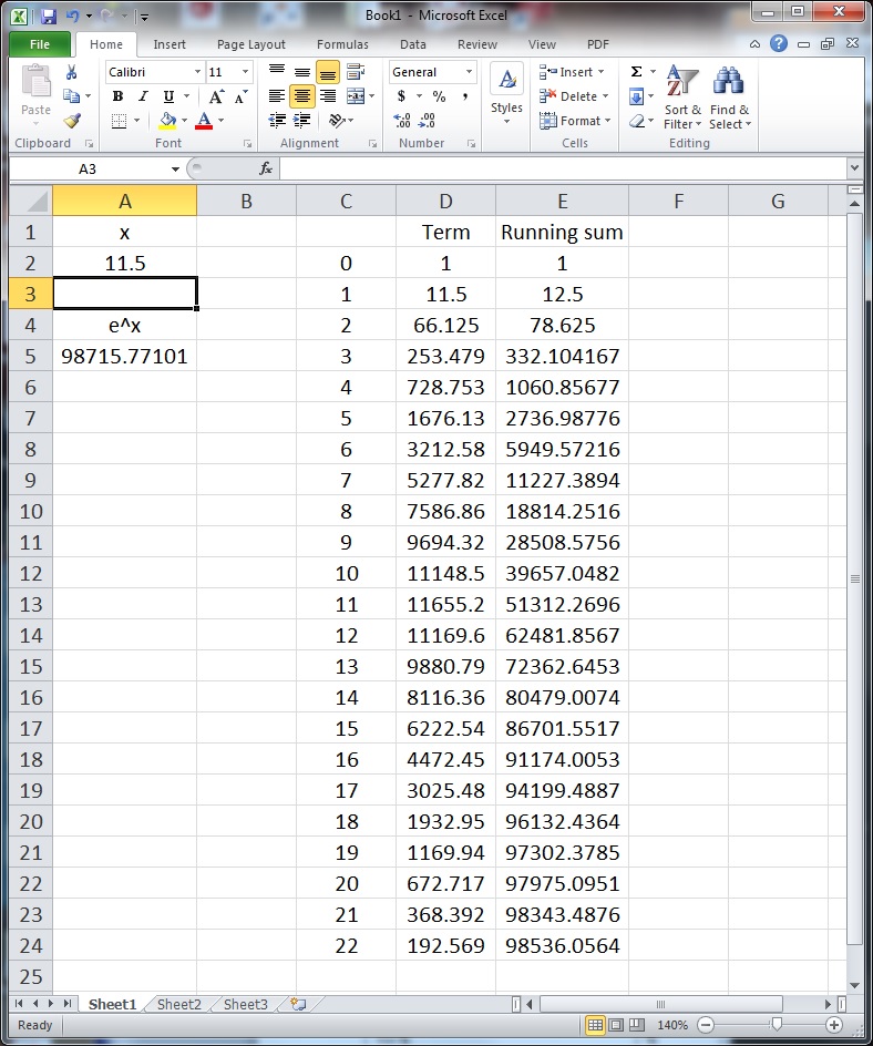
Pedagogically, I like to use a spreadsheet like Microsoft Excel to demonstrate the rate of convergence. A calculator could be used, but students can see quickly with Excel how quickly (or slowly) the terms get smaller. I usually construct the spreadsheet in class on the fly (the fill down feature is really helpful for doing this quickly), with the end product looking something like this:

In this way, students can immediately see that the Taylor series is accurate to four significant digits by going up to the $x^4$ term and that about ten or eleven terms are needed to get a figure that is as accurate as the precision of the computer will allow. In other words, for all practical purposes, an infinite number of terms are not necessary.

In short, this is how a calculator computes $e^x$ : adding up the first few terms of a Taylor series. Back in high school, when students hit the $e^x$ button on their calculators, they’ve trusted the result but the mechanics of how the calculator gets the result was shrouded in mystery. No longer.

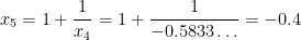
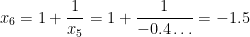
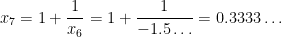
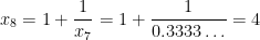
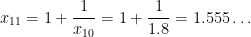
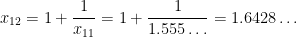
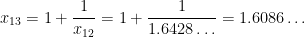
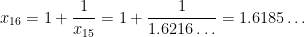
Then I shift gears by trying a larger value of $x$ :

I ask my students the obvious question: What went wrong? They’re usually able to volunteer a few ideas:

The convergence is slower for larger values of $x$ .
The series will converge, but more terms are needed (and I’ll later use the fill down feature to get enough terms so that it does converge as accurate as double precision will allow).
The individual terms get bigger until $k=11$ and then start getting smaller. I’ll ask my students why this happens, and I’ll eventually get an explanation like

$\displaystyle \frac{(11.5)^6}{6!} < \frac{(11.5)^6}{6!} \times \frac{11.5}{7} = \frac{(11.5)^7}{7!}$

but

$\displaystyle \frac{(11.5)^{11}}{11!} < \frac{(11.5)^{11}}{11!} \times \frac{11.5}{12} = \frac{(11.5)^{12}}{12!}$

At this point, I’ll mention that calculators use some tricks to speed up convergence. For example, the calculator can simply store a few values of $e^x$ in memory, like $e^{16}$ , $e^{8}$ , $e^{4}$ , $e^{2}$ , and $e^{1} = e$ . I then ask my class how these could be used to find $e^{11.5}$ . After some thought, they will volunteer that

$e^{11.5} = e^8 \cdot e^2 \cdot e \cdot e^{0.5}$ .

The first three values don’t need to be computed — they’ve already been stored in memory — while the last value can be computed via Taylor series. Also, since $0.5 < 1$ , the series for $e^{0.5}$ will converge pretty quickly. (Some students may volunteer that the above product is logically equivalent to turning $11$ into binary.)

At this point — after doing these explicit numerical examples — I’ll show graphs of $e^x$ and graphs of the Taylor polynomials of $e^x$ , observing that the polynomials get closer and closer to the graph of $e^x$ as more terms are added. (For example, see the graphs on the Wikipedia page for Taylor series, though I prefer to use Mathematica for in-class purposes.) In my opinion, the convergence of the graphs only becomes meaningful to students only after doing some numerical examples, as done above.

At this point, I hope my students are familiar with the definition of Taylor (Maclaurin) series, can apply the definition to $e^x$ , and have some intuition meaning that the nasty Taylor series expression practically means add a bunch of terms together until you’re satisfied with the convergence.

In the next post, we’ll consider another Taylor series which ought to be (but usually isn’t) really familiar to students: an infinite geometric series.

P.S. Here’s the Excel spreadsheet that I used to make the above figures: Taylor.

Reminding students about Taylor series (Part 3)

Sadly, at least at my university, Taylor series is the topic that is least retained by students years after taking Calculus II. They can remember the rules for integration and differentiation, but their command of Taylor series seems to slip through the cracks. In my opinion, the reason for this lack of retention is completely understandable from a student’s perspective: Taylor series is usually the last topic covered in a semester, and so students learn them quickly for the final and quickly forget about them as soon as the final is over.

Of course, when I need to use Taylor series in an advanced course but my students have completely forgotten this prerequisite knowledge, I have to get them up to speed as soon as possible. Here’s the sequence that I use to accomplish this task. Covering this sequence usually takes me about 30 minutes of class time.

I should emphasize that I present this sequence in an inquiry-based format: I ask leading questions of my students so that the answers of my students are driving the lecture. In other words, I don’t ask my students to simply take dictation. It’s a little hard to describe a question-and-answer format in a blog, but I’ll attempt to do this below.

In the previous post, I described how I lead students to the equations

$f(x) = \displaystyle \sum_{k=0}^n \frac{f^{(k)}(0)}{k!} x^k$ .

and

$f(x) = \displaystyle \sum_{k=0}^n \frac{f^{(k)}(a)}{k!} (x-a)^k$ ,

where $f(x)$ is a polynomial and $a$ can be any number.

Step 3. What happens if the original function $f(x)$ is not a polynomial? For one thing, the right-hand side can no longer be a finite sum. As long as the sum on the right-hand side stops at some degree $n$ , the right-hand side is a polynomial, but the left-hand side is assumed to not be a polynomial.

To resolve this, we can cross our fingers and hope that

$f(x) = \displaystyle \sum_{k=0}^{\infty} \frac{f^{(k)}(0)}{k!} x^k$ ,

$f(x) = \displaystyle \sum_{k=0}^{\infty}\frac{f^{(k)}(a)}{k!} (x-a)^k$ .

In other words, let’s make the right-hand side an infinite series, and hope for the best. This is the definition of the Taylor series expansions of $f$ .

Note: At this point in the review, I can usually see the light go on in my students’ eyes. Usually, they can now recall their work with Taylor series in the past… and they wonder why they weren’t taught this topic inductively (like I’ve tried to do in the above exposition) instead of deductively (like the presentation in most textbooks).

While we’d like to think that the Taylor series expansions always work, there are at least two things that can go wrong.

First, the sum on the left is an infinite series, and there’s no guarantee that the series will converge in the first place. There are plenty of example of series that diverge, like $\displaystyle \sum_{k=0}^\infty \frac{1}{k+1}$ .
Second, even if the series converges, there’s no guarantee that the series will converge to the “right” answer $f(x)$ . The canonical example of this behavior is $f(x) = e^{-1/x^2}$ , which is so “flat” near $x=0$ that every single derivative of $f$ is equal to $0$ at $x =0$ .

For the first complication, there are multiple tests devised in Calculus II, especially the Ratio Test, to determine the values of $x$ for which the series converges. This establishes a radius of convergence for the series.

The second complication is far more difficult to address rigorously. The good news is that, for all commonly occurring functions in the secondary mathematics curriculum, the Taylor series of a function properly converges (when it does converge). So we will happily ignore this complication for the remainder of the presentation.

Indeed, it’s remarkable that the series should converge to $f(x)$ at all. Think about the meaning of the terms on the right-hand side:

$f(a)$ is the $y-$ coordinate at $x=a$ .
$f'(a)$ is the slope of the curve at $x=a$ .
$f''(a)$ is a measure of the concavity of the curve at — you guessed it — $x=a$ .
$f'''(a)$ is an even more subtle description of the curve… once again, at $x=a$ .

In other words, if the Taylor series converges to $f(x)$ , then every twist and turn of the function, even at points far away from $x=a$ , is encoded somehow in the shape of the curve at the one point $x=a$ . So analytic functions (which has a Taylor series which converges to the original functions) are indeed quite remarkable.