Engaging students: Using right-triangle trigonometry

In my capstone class for future secondary math teachers, I ask my students to come up with ideas for engaging their students with different topics in the secondary mathematics curriculum. In other words, the point of the assignment was not to devise a full-blown lesson plan on this topic. Instead, I asked my students to think about three different ways of getting their students interested in the topic in the first place.

I plan to share some of the best of these ideas on this blog (after asking my students’ permission, of course).

This student submission comes from my former student Shama Surani. Her topic, from Precalculus: using right-triangle trigonometry.

How could you as a teacher create an activity or project that involves your topic?

A project that Dorathy Scrudder, Sam Smith, and I did that involves right-triangle trigonometry in our PBI class last week, was to have the students to build bridges. Our driving question was “How can we redesign the bridge connecting I-35 and 635?” The students knew that the hypotenuse would be 34 feet, because there were two lanes, twelve feet each, and a shoulder of ten feet that we provided on a worksheet. As a group, they needed to decide on three to four angles between 10-45 degrees, and calculate the sine and cosine of the angle they chose. One particular group used the angle measures of 10°, 20°, 30°, and 40°. They all calculated the sine of their angles to find the height of the triangle, and used cosine to find the width of their triangle by using 34 as their hypotenuse. The picture above is by Sam Smith, and it illustrates the triangles that we wanted the students to calculate.

The students were instructed to make a scale model of a bridge so they were told that 1 feet = 0.5 centimeters. Hence, the students had to divide all their calculations by two. Then, the students had to check their measurements of their group members, and were provided materials such as cardstock, scissors, pipe cleaners, tape, rulers, and protractors in order to construct their bridges. They had to use a ruler to measure out what they found for sine and cosine on the cardstock, and make sure when they connected the line to make the hypotenuse that the hypotenuse had a length of 17 centimeters. After they drew their triangles, they had to use a protractor to verify that the angle they chose is what one of the angles were in the triangle. When our students presented, they were able to communicate what sine and cosine represented, and grasped the concepts.

Below are pictures of the triangles and bridges that one of our groups of students constructed. Overall, the students enjoyed this project, and with some tweaks, I believe this will be an engaging project for right triangle trigonometry.

How does this topic extend what your students should have learned in previous courses?

In previous classes, such in geometry, students should have learned about similar and congruent triangles in addition to triangle congruence such as side-side-side and side-angle-side. They should also have learned if they have a right angle triangle, and they are given two sides, they can find the other side by using the Pythagorean Theorem. The students should also have been exposed to special right triangles such as the 45°-45°-90° triangles and 30°-60°-90° triangles and the relationships to the sides. Right triangle trigonometry extends the ideas of these previous classes. Students know that there must be a 45°-45°-90° triangle has side lengths of 1, 1, and $\sqrt{2}$ which the lengths of 1 subtending the 45° angles. They also are aware that a 30°-60°-90° produces side lengths of 1, $\sqrt{3}$ , and 2, with the side length of 1 subtending the 30°, the length of $\sqrt{3}$ subtending the angle of 60°, and the length of 2 subtending the right angle. So, what happens when there is a right angle triangle, but the other two angles are not 45 degrees or 30 and 60 degrees? This is where right triangle trigonometry comes into play. Students will now be able to calculate the sine, cosine, and tangent and its reciprocal functions for those triangles that are right. Later, this topic will be extended to the unit circle and graphing the trigonometric functions as well as their reciprocal functions and inverse functions.

What are the contributions of various cultures to this topic?

Below are brief descriptions of various cultures that personally interested me.

Early Trigonometry

The Babylonians and Egyptians studied the sides of triangles other than angle measure since the concept of angle measure was not yet discovered. The Babylonian astronomers had detailed records on the rising and setting of stars, the motion of planets, and the solar and lunar eclipses. On the other hand, Egyptians used a primitive form of trigonometry in order to build the pyramids.

Greek Mathematics

Hipparchus of Nicaea, now known as the father of Trigonometry, compiled the first trigonometric table. He was the first one to formulate the corresponding values of arc and chord for a series of angles. Claudius Ptolemy wrote Almagest, which expanded on the ideas of Hipparchus’ ideas of chords in a circle. The Almagest is about astronomy, and astronomy relies heavily on trigonometry.

Indian Mathematics

Influential works called Siddhantas from the 4^th-5^th centry, first defined sine as the modern relationship between half an angle and half a chord. It also defined cosine, versine (which is 1 – cosine), and inverse sine. Aryabhata, an Indian astronomer and mathematician, expanded on the ideas of Siddhantas in another important work known as Aryabhatiya. Both of these works contain the earliest surviving tables of sine and versine values from 0 to 90 degrees, accurate to 4 decimal places. Interestingly enough, the words jya was for sine and kojya for cosine. It is now known as sine and cosine due to a mistranslation.

Islamic Mathematics

Muhammad ibn Mūsā al-Khwārizmī had produced accurate sine and cosine tables in the 9^th century AD. Habash al-Hasib al-Marwazi was the first to produce the table of cotangents in 830 AD. Similarly, Muhammad ibn Jābir al-Harrānī al-Battānī had discovered the reciprocal functions of secant and cosecant. He also produced the first table of cosecants.

Muslim mathematicians were using all six trigonometric functions by the 10^th century. In fact, they developed the method of triangulation which helped out with geography and surveying.

Chinese Mathematics

In China, early forms of trigonometry were not as widely appreciated as it was with the Greeks, Indians, and Muslims. However, Chinese mathematicians needed spherical geometry for calendrical science and astronomical calculations. Guo Shoujing improved the calendar system and Chinese astronomy by using spherical trigonometry in his calculations.

European Mathematics

Regiomontanus treated trigonometry as a distinct mathematical discipline. A student of Copernicus, Georg Joachim Rheticus, was the first one to define all six trigonometric functions in terms of right triangles other than circles in Opus palatinum de triangulis. Valentin Otho finished his work in 1596.

http://en.wikipedia.org/wiki/History_of_trigonometry

Functions that commute

At the bottom of this post is a one-liner that I use in my classes the first time I present a theorem where two functions are permitted to commute. At many layers of the mathematics curriculum, students learn about that various functions can essentially commute with each other. In other words, the order in which the operations is performed doesn’t affect the final answer. Here’s a partial list off the top of my head:

Arithmetic/Algebra: $a \cdot (b + c) = a \cdot b + a \cdot c$ . This of course is commonly called the distributive property (and not the commutative property), but the essential idea is that the same answer is obtained whether the multiplications are performed first or if the addition is performed first.
Algebra: If $a,b > 0$ , then $\sqrt{ab} = \sqrt{a} \sqrt{b}$ .
Algebra: If $a,b > 0$ and $x$ is any real number, then $(ab)^x = a^x b^x$ .
Precalculus: $\displaystyle \sum_{i=1}^n (a_i+b_i) = \displaystyle \sum_{i=1}^n a_i + \sum_{i=1}^n b_i$ .
Precalculus: $\displaystyle \sum_{i=1}^n c a_i = c \displaystyle \sum_{i=1}^n a_i$ .
Calculus: If $f$ is continuous at an interior point $c$ , then $\displaystyle \lim_{x \to c} f(x) = f(c)$ .
Calculus: If $f$ and $g$ are differentiable, then $(f+g)' = f' + g'$ .
Calculus: If $f$ is differentiable and $c$ is a constant, then $(cf)' = cf'$ .
Calculus: If $f$ and $g$ are integrable, then $\int (f+g) = \int f + \int g$ .
Calculus: If $f$ is integrable and $c$ is a constant, then $\int cf = c \int f$ .
Calculus: If $f: \mathbb{R}^2 \to \mathbb{R}$ is integrable, $\iint f(x,y) dx dy = \iint f(x,y) dy dx$ .
Calculus: For most differentiable function $f: \mathbb{R}^2 \to \mathbb{R}$ that arise in practice, $\displaystyle \frac{\partial^2 f}{\partial x \partial y} = \displaystyle \frac{\partial^2 f}{\partial y \partial x}$ .
Probability: If $X$ and $Y$ are random variables, then $E(X+Y) = E(X) + E(Y)$ .
Probability: If $X$ is a random variable and $c$ is a constant, then $E(cX) = c E(X)$ .
Probability: If $X$ and $Y$ are independent random variables, then $E(XY) = E(X) E(Y)$ .
Probability: If $X$ and $Y$ are independent random variables, then $\hbox{Var}(X+Y) = \hbox{Var}(X) + \hbox{Var}(Y)$ .
Set theory: If $A$ , $B$ , and $C$ are sets, then $A \cup (B \cap C) = (A \cup B) \cap (A \cup C)$ .
Set theory: If $A$ , $B$ , and $C$ are sets, then $A \cap (B \cup C) = (A \cap B) \cup (A \cap C)$ .

However, there are plenty of instances when two functions do not commute. Most of these, of course, are common mistakes that students make when they first encounter these concepts. Here’s a partial list off the top of my head. (For all of these, the inequality sign means that the two sides do not have to be equal… though there may be special cases when equality happens to happen.)

Algebra: $(a+b)^x \ne a^x + b^x$ if $x \ne 1$ . Important special cases are $x = 2$ , $x = 1/2$ , and $x = -1$ .
Algebra/Precalculus: $\log_b(x+y) = \log_b x + \log_b y$ . I call this the third classic blunder.
Precalculus: $(f \circ g)(x) \ne (g \circ f)(x)$ .
Precalculus: $\sin(x+y) \ne \sin x + \sin y$ , $\cos(x+y) \ne \cos x + \cos y$ , etc.
Precalculus: $\displaystyle \sum_{i=1}^n (a_i b_i) \ne \displaystyle \left(\sum_{i=1}^n a_i \right) \left( \sum_{i=1}^n b_i \right)$ .
Calculus: $(fg)' \ne f' \cdot g'$ .
Calculus $\left( \displaystyle \frac{f}{g} \right)' \ne \displaystyle \frac{f'}{g'}$
Calculus: $\int fg \ne \left( \int f \right) \left( \int g \right)$ .
Probability: If $X$ and $Y$ are dependent random variables, then $E(XY) \ne E(X) E(Y)$ .
Probability: If $X$ and $Y$ are dependent random variables, then $\hbox{Var}(X+Y) \ne \hbox{Var}(X) + \hbox{Var}(Y)$ .

All this to say, it’s a big deal when two functions commute, because this doesn’t happen all the time.

I wish I could remember the speaker’s name, but I heard the following one-liner at a state mathematics conference many years ago, and I’ve used it to great effect in my classes ever since. Whenever I present a property where two functions commute, I’ll say, “In other words, the order of operations does not matter. This is a big deal, because, in real life, the order of operations usually is important. For example, this morning, you probably got dressed and then went outside. The order was important.”

Calculators and complex numbers (Part 24)

In this series of posts, I explore properties of complex numbers that explain some surprising answers to exponential and logarithmic problems using a calculator (see video at the bottom of this post). These posts form the basis for a sequence of lectures given to my future secondary teachers.

To begin, we recall that the trigonometric form of a complex number $z = a+bi$ is

$z = r(\cos \theta + i \sin \theta) = r e^{i \theta}$

where $r = |z| = \sqrt{a^2 + b^2}$ and $\tan \theta = b/a$ , with $\theta$ in the appropriate quadrant. As noted before, this is analogous to converting from rectangular coordinates to polar coordinates.

Theorem. If $z = x + i y$ , where $x$ and $y$ are real numbers, then

$e^z = e^x (\cos y + i \sin y)$

Definition. Let $z = r e^{i \theta}$ be a complex number so that $-\pi < \theta \le \theta$ . Then we define

$\log z = \ln r + i \theta$ .

Definition. Let $z$ and $w$ be complex numbers so that $z \ne 0$ . Then we define

$z^w = e^{w \log z}$

Technical point: for the latter two definitions, these are the principal values of the functions. In complex analysis, these are usually considered multiply-defined functions. But I’m not going to worry about this technicality here and will only consider the principal values.

This is the last post in this series, where I state some generalizations of the Laws of Exponents for complex numbers.

In yesterday’s post, we saw that $z^{w_1} z^{w_2} = z^{w_1 + w_2}$ as long as $z \ne 0$ . This prevents something like $0^4 \cdot 0^{-3} = 0^1$ , since $0^{-3}$ is undefined.

Theorem. Let $z \in \mathbb{C} \setminus \{ 0 \}$ , $w \in \mathbb{C}$ , and $n \in \mathbb{Z}$ . Then $(z^w)^n = z^{wn}$ .

As we saw in a previous post, the conclusion could be incorrect outside of the above hypothesis, as $\displaystyle \left[ (-1)^3 \right]^{1/2} \ne (-1)^{3/2}$ .

Theorem. Let $u \in \mathbb{R}$ and $z \in \mathbb{C}$ . Then $(e^u)^z = e^{uz}$ .

Theorem. Let $x, y > 0$ be real numbers and $z \in \mathbb{C}$ . Then $x^z y^z = (xy)^z$ .

Again, the conclusion of the above theorem could be incorrect outside of these hypothesis, as $(-2)^{1/2} (-3)^{1/2} \ne \left[ (-2) \cdot (-3) \right]^{1/2}$ .

green line

For completeness, here’s the movie that I use to engage my students when I begin this sequence of lectures.

Calculators and complex numbers (Part 23)

To begin, we recall that the trigonometric form of a complex number $z = a+bi$ is

$z = r(\cos \theta + i \sin \theta) = r e^{i \theta}$

Theorem. If $z = x + i y$ , where $x$ and $y$ are real numbers, then

$e^z = e^x (\cos y + i \sin y)$

Definition. Let $z = r e^{i \theta}$ be a complex number so that $-\pi < \theta \le \theta$ . Then we define

$\log z = \ln r + i \theta$ .

Definition. Let $z$ and $w$ be complex numbers so that $z \ne 0$ . Then we define

$z^w = e^{w \log z}$

In the remaining posts in this series, I want to explore which properties of exponential functions remain true when complex numbers are used.

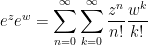
To begin, if $w$ is a real rational number, then there is an alternative definition of $z^w$ that matches De Moivre’s Theorem. Happily, the two definitions agree. Suppose that $z = r e^{i \theta}$ with $-\pi < \theta \le \pi$ . Then

$z^w = e^{w \log z}$

$= e^{w [\ln r + i \theta]}$

$= e^{w \ln r + i w \theta}$

$= e^{w \ln r} e^{i w \theta}$

$= r^w (\cos w\theta + i \sin \theta)$

Next, one of the Laws of Exponents remains true even for complex numbers:

$z^{w_1} z^{w_2} = e^{w_1 \log z} e^{w_2 \log z}$

$= e^{w_1 \log z + w_2 \log z}$

$= e^{(w_1 + w_2) \log z}$

$= z^{w_1 + w_2}$ .

However, in previous posts, we’ve seen that the rules $(x^y)^z = x^(yz)$ and $x^z y^z = (xy)^z$ may not be true if nonpositive bases, let alone complex bases, are used.

We can also derive the usual rules $z^0 = 1$ and $z^{-w} = \displaystyle \frac{1}{z^w}$ . First,

$z^0 = e^{0 \log z} = e^0 = 1$ .

Next, we think like an MIT freshman and use the above Law of Exponents to observe that

$z^w z^{-w} = z^{w-w} = z^0 = 1$ .

Dividing, we see that $z^{-w} = \displaystyle \frac{1}{z^w}$ .

green line

For completeness, here’s the movie that I use to engage my students when I begin this sequence of lectures.

Calculators and complex numbers (Part 22)

To begin, we recall that the trigonometric form of a complex number $z = a+bi$ is

$z = r(\cos \theta + i \sin \theta) = r e^{i \theta}$

Theorem. If $z = x + i y$ , where $x$ and $y$ are real numbers, then

$e^z = e^x (\cos y + i \sin y)$

Definition. Let $z = r e^{i \theta}$ be a complex number so that $-\pi < \theta \le \theta$ . Then we define

$\log z = \ln r + i \theta$ .

At long last, we are now in position to explain the last surprising results from the calculator video below.

Definition. Suppose that $z$ and $w$ are complex numbers so that $z \ne 0$ . Then we define

$z^w = e^{w \log z}$

Naturally, this definition makes sense if $z$ and $w$ are real numbers.

For example, let’s consider the computation of $i^i$ . For the base of $i$ , we note that

$\log i = \log e^{\pi i/ 2} = \displaystyle \frac{\pi i}{2}$ .

Therefore,

$i^i = e^{i \log i} = e^{i \pi i/2} = e^{-\pi/2}$ ,

which is (surprisingly) a real number.

As a second example, let’s compute $(-8)^i$ . To begin,

$\log(-8) = \log \left( 8 e^{\pi i} \right) = \ln 8 + \pi i$ .

Therefore,

$(-8)^i = e^{i \log(-8)}$

$= e^{i (\ln 8 + \pi i)}$

$= e^{-\pi + i \ln 8}$

$= e^{-\pi} (\cos [\ln 8] + i \sin [ \ln 8 ] )$

$= e^{-\pi} \cos (\ln 8) + i e^{-\pi} \sin (\ln 8)$

In other words, a problem like this is a Precalculus teacher’s dream come true, as it contains $e, \ln, \pi, \cos, \sin$ , and $i$ in a single problem.

green line

For completeness, here’s the movie that I use to engage my students when I begin this sequence of lectures.

Calculators and complex numbers (Part 21)

To begin, we recall that the trigonometric form of a complex number $z = a+bi$ is

$z = r(\cos \theta + i \sin \theta) = r e^{i \theta}$

Over the past few posts, we developed the following theorem for computing $e^z$ in the case that $z$ is a complex number.

Definition. Let $z = r e^{i \theta}$ be a complex number so that $-\pi < \theta \le \theta$ . Then we define

$\log z = \ln r + i \theta$ .

Of course, this looks like what the definition ought to be if one formally applies the Laws of Logarithms to $r e^{i \theta}$ . However, this complex logarithm doesn’t always work the way you’d think it work. For example,

$\log \left(e^{2 \pi i} \right) = \log (\cos 2\pi + i \sin 2\pi) = \log 1 = \ln 1 = 0 \ne 2\pi i$ .

This is analogous to another situation when an inverse function is defined using a restricted domain, like

$\sqrt{ (-3)^2 } = \sqrt{9} = 3 \ne -3$

$\sin^{-1} (\sin \pi) = \sin^{-1} 0 = 0 \ne \pi$ .

The Laws of Logarithms also may not work when nonpositive numbers are used. For example,

$\log \left[ (-1) \cdot (-1) \right] = \log 1 = 0$ ,

but

$\log(-1) + \log(-1) = \log \left( e^{\pi i} \right) + \log \left( e^{\pi i} \right) = \pi i + \pi i = 2\pi i$ .

green line

For completeness, here’s the movie that I use to engage my students when I begin this sequence of lectures.

Calculators and complex numbers (Part 20)

To begin, we recall that the trigonometric form of a complex number $z = a+bi$ is

$z = r(\cos \theta + i \sin \theta) = r e^{i \theta}$

Over the past few posts, we developed the following theorem for computing $e^z$ in the case that $z$ is a complex number.

Theorem. If $z = x + i y$ , where $x$ and $y$ are real numbers, then

$e^z = e^x (\cos y + i \sin y)$

As a consequence, there are infinitely many complex solutions of the equation

$e^z = -2 - 2i$ ,

namely, $z = \ln 2\sqrt{2} - \displaystyle \frac{3\pi}{4} + 2 \pi n i$ .

Choosing the solution that has an imaginary part in the interval $(-\pi,\pi]$ leads to the definition of the complex logarithm.

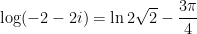
Definition. Let $z = r e^{i \theta}$ be a complex number so that $-\pi < \theta \le \theta$ . Then we define

$\log z = \ln r + i \theta$ .

Of course, this looks like what the definition ought to be if one formally applies the Laws of Logarithms to $r e^{i \theta}$ . So, for example,

$\log (-2-2i) = \ln 2\sqrt{2} - \displaystyle \frac{3\pi}{4}$

A technicality: this is the principal value of the complex logarithm. In complex analysis, this is technically thought of as a multiply-defined function.

The complex version of the natural logarithm function matches the ordinary definition when applied to real numbers. For example,

$\log 6 = \log \left( 6 e^{0i} \right) = \ln 6 + 0 i = \ln 6$ .

A couple of observations. In high school, the symbol $\log$ is usually dedicated to base 10. However, in higher-level mathematics courses, $\log$ always means natural logarithm. That’s because, for the purposes of abstract mathematics, base-10 logarithms are practically useless. They are helpful for us people since our number system uses base 10; it’s easy for me to estimate $\log_{10} 9000$ , but $\ln 9000$ requires a little more thought. But nearly all major theorems that involve logarithms specifically employ natural logarithms. Indeed, when I first become a professor, I had to remind myself that my students used $\ln$ for natural logarithms and not $\log$ . Still, I write $\log_{10}$ for base-10 logarithms and not $\log$ as a silent acknowledgment of the use of the symbol in higher-level courses.

This use of the logarithm explains the final results of the calculator in the video below. When $\ln(-5)$ is entered, it assumes that a real answer is expected, and so the calculatore returns an error message. On the other hand, when $\ln(-5+0i)$ is entered, it assumes that the user wants the principal complex logarithm. Since $-5+0i = 5 e^{i \pi}$ , the calculator correctly returns $\ln 5 + \pi i$ as the answer. (Of course, the calculator still uses $\ln$ and not $\log$ to mean natural logarithm.)

green line

For completeness, here’s the movie that I use to engage my students when I begin this sequence of lectures.

Calculators and complex numbers (Part 19)

To begin, we recall that the trigonometric form of a complex number $z = a+bi$ is

$z = r(\cos \theta + i \sin \theta) = r e^{i \theta}$

Over the past few posts, we developed the following theorem for computing $e^z$ in the case that $z$ is a complex number.

Theorem. If $z = x + i y$ , where $x$ and $y$ are real numbers, then

$e^z = e^x (\cos y + i \sin y)$

Example. Find all complex numbers $z$ so that $e^z = 5$ .

Solution. If $z = x + iy$ , then

$e^x (\cos y + i \sin y) = 5 (\cos 0 + i \sin 0)$

Matching parts, we see that $e^x = 5$ and that the angle $y$ must be coterminal with $0$ radians. In other words,

$x = \ln 5 \qquad$ and $\qquad y = 2\pi n$ for any integer $n$ .

Therefore, there are infinitely many answers: $z = \ln 5 + 2 \pi n i$ .

Notice that there’s nothing particularly special about the number $5$ . This could have been any nonzero number, including complex numbers, and there still would have been an infinite number of solutions. (This is completely analogous to solving a trigonometric equation like $\sin \theta = 1$ , which similarly has an infinite number of solutions.) For example, the complex solutions of the equation

$e^z = -2 - 2i$

are $z = \ln 2\sqrt{2} - \displaystyle \frac{3\pi}{4} + 2 \pi n i$ .

These observations lead to the following theorems, which I’ll state without proof.

Theorem. The range of the function $f(z) = e^z$ is $\mathbb{C} \setminus \{ 0 \}$ .

Theorem. $e^z = e^w \Longleftrightarrow z = w + 2\pi n i$ .

Naturally, these conclusions are different than the normal case when $z$ is assumed to be a real number.

green line

For completeness, here’s the movie that I use to engage my students when I begin this sequence of lectures.

Calculators and complex numbers (Part 18)

To begin, we recall that the trigonometric form of a complex number $z = a+bi$ is

$z = r(\cos \theta + i \sin \theta) = r e^{i \theta}$

Definition. If $z$ is a complex number, then we define

$e^z = \displaystyle \sum_{n=0}^{\infty} \frac{z^n}{n!}$

This of course matches the Taylor expansion of $e^x$ for real numbers $x$ .

In the last few posts, we proved the following theorem.

Theorem. If $z$ and $w$ are complex numbers, then $e^z e^w = e^{z+w}$.

This theorem allows us to compute $e^z$ without directly plugging into the above infinite series.

Theorem. If $z = x + i y$ , where $x$ and $y$ are real numbers, then

$e^z = e^x (\cos y + i \sin y)$

Proof. With the machinery that’s been developed over the past few posts, this one is actually a one-liner:

$e^z = e^{x+iy} = e^x e^{iy} = e^x (\cos y + i \sin y)$ .

For example,

$e^{4+\pi i} = e^4 (\cos \pi + i \sin \pi) = -e^4$

Notice that, with complex numbers, it’s perfectly possible to take $e$ to a power and get a negative number. Obviously, this is impossible when using only real numbers.

Another example:

$e^{-2+3i} = e^{-2} (\cos 3 +i \sin 3)$

In this answer, we have to remember that the angle is 3 radians and not 3 degrees.

green line

For completeness, here’s the movie that I use to engage my students when I begin this sequence of lectures.

Calculators and complex numbers (Part 17)

Definition. If $z$ is a complex number, then we define

$e^z = \displaystyle \sum_{n=0}^{\infty} \frac{z^n}{n!}$

Even though this isn’t the usual way of defining the exponential function for real numbers, the good news is that one Law of Exponents remains true. (At we saw in an earlier post in this series, we can’t always assume that the usual Laws of Exponents will remain true when we permit the use of complex numbers.)

Theorem. If $z$ and $w$ are complex numbers, then $e^z e^w = e^{z+w}$ .

In yesterday’s post, I gave the idea behind the proof… group terms where the sums of the exponents of $z$ and $w$ are the same. Today, I will formally prove the theorem.

The proof of the theorem relies on a principle that doesn’t seem to be taught very often anymore… rearranging the terms of a double sum. In this case, the double sum is

$e^z e^w = \displaystyle \sum_{n=0}^{\infty} \sum_{k=0}^{\infty} \frac{z^n}{n!} \frac{w^k}{k!}$

This can be visualized in the picture below, where the $x-$ axis represents the values of $k$ and the $y-$ axis represents the values of $n$ . Each red dot symbolizes a term in the above double sum. For a fixed value of $n$ , the values of $k$ vary from $0$ to $\infty$ . In other words, we start with $n =0$ and add all the terms on the line $n = 0$ (i.e., the $x-$ axis in the picture). Then we go up to $n = 1$ and then add all the terms on the next horizontal line. And so on.

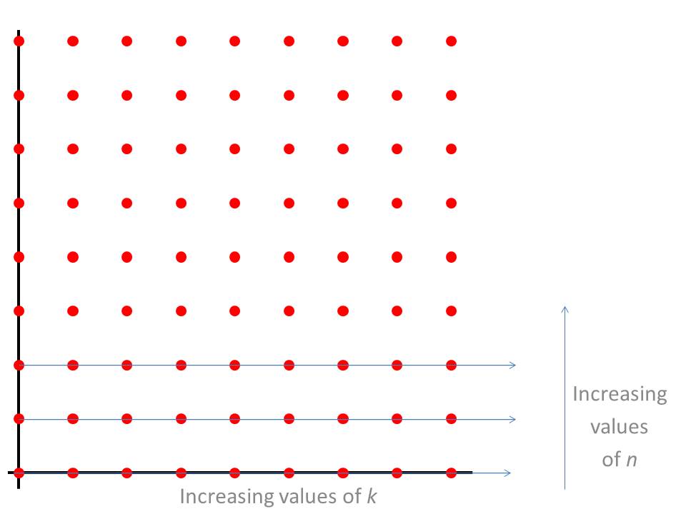
I will rearrange the terms as follows: Let $j = n+k$ . Then for a fixed value of $j$ , the values of $k$ will vary from $0$ to $j$ . This is perhaps best described in the picture below. The value of $j$ , the sum of the coordinates, is constant along the diagonal lines below. The value of $k$ then changes while moving along a diagonal line.

Even though this is a different way of adding the terms, we clearly see that all of the red circles will be hit regardless of which technique is used for adding the terms.

In this way, the double sum $\displaystyle \sum_{n=0}^\infty \sum_{k=0}^\infty$ gets replaced by $\displaystyle \sum_{j=0}^\infty \sum_{k=0}^j$ . Since $n = j-k$ , we have

$e^z e^w = \displaystyle \sum_{j=0}^{\infty} \sum_{k=0}^{j} \frac{z^{j-k}}{(j-k)!} \frac{w^k}{k!}$

We now add a couple of $j!$ terms to this expression for reasons that will become clear shortly:

$e^z e^w = \displaystyle \sum_{j=0}^{\infty} \sum_{k=0}^{j} \frac{j!}{j!} \frac{1}{k! (j-k)!} w^k z^{j-k}$

Since $j!$ does not contain any $k$ s, it can be pulled outside of the inner sum on $k$ . We do this for the $j!$ in the denominator:

$= \displaystyle \sum_{j=0}^\infty \frac{1}{j!} \sum_{k=0}^j \frac{j!}{k!(j-k)!} w^k z^{j-k}$

We recognize that $\displaystyle \frac{j!}{k! (j-k)!}$ is a binomial coefficent:

$= \displaystyle \sum_{j=0}^\infty \frac{1}{j!} \sum_{k=0}^j {j \choose k} w^k z^{j-k}$

The inner sum is recognized as the formula for a binomial expansion:

$= \displaystyle \sum_{j=0}^\infty \frac{1}{j!} (w+z)^j$

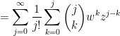
Finally, we recognize this as the definition of $e^{w+z}$ , using the dummy variable $j$ instead of $n$ . This proves that $e^z e^w = e^{z+w}$ even if $z$ and $w$ are complex.

Without a doubt, this theorem was a lot of work. The good news is that, with this result, it will no longer be necessary to explicitly use the summation definition of $e^z$ to actually compute $e^z$ , as we’ll see tomorrow.

green line For completeness, here’s the movie that I use to engage my students when I begin this sequence of lectures.