In this series of posts, we have seen that the number  can be thought about in three different ways.
1. defines a region of area 1 under the hyperbola  .
. 2. We have the limits
 .
.
These limits form the logical basis for the continuous compound interest formula.
3. We have also shown that  . From this derivative, the Taylor series expansion for
  about
about  can be computed:

Therefore, we can let  to find :


Let’s now consider how the decimal expansion of might be obtained from these three different methods.
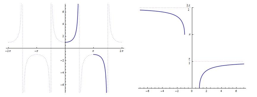
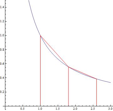
1. Finding using only the original definition is a genuine pain in the neck. The only way to approximate is by trapping the value of using various approximation. For example, consider the picture below, showing the curve and trapezoidal approximations on the intervals ![[1,1.8]](https://s0.wp.com/latex.php?latex=%5B1%2C1.8%5D&bg=ffffff&fg=000000&s=0&c=20201002) and
and ![[1.8,2.6]](https://s0.wp.com/latex.php?latex=%5B1.8%2C2.6%5D&bg=ffffff&fg=000000&s=0&c=20201002) . (Because I need a good picture, I used Mathematica and not Microsoft Paint.)
. (Because I need a good picture, I used Mathematica and not Microsoft Paint.)

Each trapezoid has a (horizontal) height of  . Furthermore, the bases of the first trapezoids have length
  and
and  , while the bases of the second trapezoid of length and
  . Notice that the trapezoids extend above the hyperbola, so that
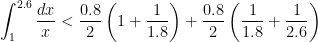

However, the number is defined to be the place where the area under the curve is exactly equal to  , and so

In other words, we know that the area between and  is strictly less than , and therefore a number larger than must be needed to obtain an area equal to .
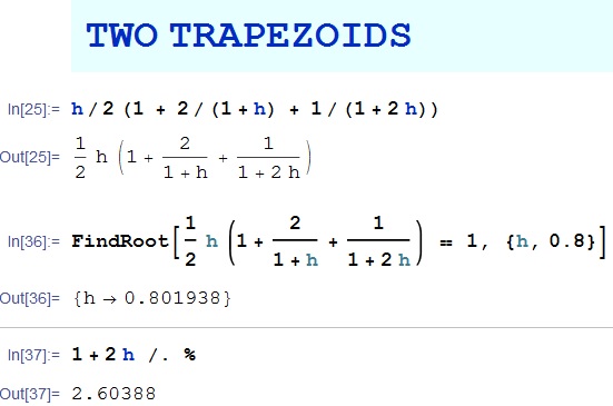
Great, so  . Can we do better? Sadly, with two equal-sized trapezoids, we can’t do much better. If the height of the trapezoids was
  and not
  , then the sum of the areas of the two trapezoids would be

By either guessing and checking — or with the help of Mathematica — it can be determined that this function of is equal to 1 at approximately  , thus establishing that
  .
.

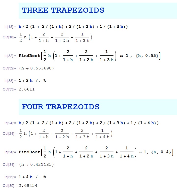
We can try to better with additional trapezoids. With four trapezoids, we can establish that  .
.

With 100 trapezoids, we can show that  .
.
 However, trapezoids can only provide a lower bound on because the original trapezoids all extend over the hyperbola.
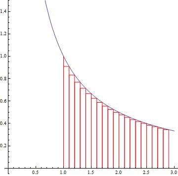
To obtain an upper bound on , we will use a lower Riemann sum to approximate the area under the curve. For example, notice the following picture of 19 rectangles of width  ranging from
  to
to  .
.
 The rectangles all lie below the hyperbola. The width of each one is , and the heights vary from
  to
to  . Therefore,
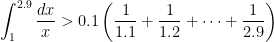

In other words, we know that the area between and  is strictly greater than , and therefore a number smaller than must be needed to obtain an area equal to . So, in a nutshell, we’ve shown that
  .
.
Once again, additional rectangles can provide better and better upper bounds on . However, since rectangles do not approximate the hyperbola as well as trapezoids, we expect the convergence to be much slower. For example, with 100 rectangles of width , the sum of the areas of the rectangles would be
It then becomes necessary to plug in numbers for until we find something that’s decently close to yet greater than . Or we can have Mathematica do the work for us:
 So with 100 rectangles, we can establish that
  . With 1000 rectangles, we can establish that
  .
.
Clearly, this is a lot of work for approximating . With all of the work shown in this post, we have shown that  , but we’re not yet sure if the next digit is
  or
or  .
.
In the next post, we’ll explore the other two ways of thinking about the number as well as their computational tractability.


![\displaystyle \int_0^4 \frac{1}{4} x^2 \, dx = \displaystyle \left[ \frac{x^3}{12} \right]^4_0](https://s0.wp.com/latex.php?latex=%5Cdisplaystyle+%5Cint_0%5E4+%5Cfrac%7B1%7D%7B4%7D+x%5E2+%5C%2C+dx+%3D+%5Cdisplaystyle+%5Cleft%5B+%5Cfrac%7Bx%5E3%7D%7B12%7D+%5Cright%5D%5E4_0&bg=ffffff&fg=000000&s=0&c=20201002)


 .
. satisfies the horizontal line test. It turns out that the choice of domain has surprising consequences that are almost unforeseeable using only the tools of Precalculus.
 uses the interval
 ![[0,\pi]](https://s0.wp.com/latex.php?latex=%5B0%2C%5Cpi%5D&bg=ffffff&fg=000000&s=0&c=20201002) — or, more precisely,
— or, more precisely, ![[0,\pi/2) \cup (\pi/2, \pi]](https://s0.wp.com/latex.php?latex=%5B0%2C%5Cpi%2F2%29+%5Ccup+%28%5Cpi%2F2%2C+%5Cpi%5D&bg=ffffff&fg=000000&s=0&c=20201002) to avoid the vertical asymptote at
to avoid the vertical asymptote at  — in order to approximately match the range of
  . However, when I was a student, I distinctly remember that my textbook chose
 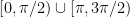 as the range for
  .
.


 . Clearly, we can replace
  with
with  is a lot simpler than we saw in yesterday’s post. Once again, we begin with one of the Pythagorean identities:
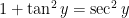


 must lie in either the interval
  or else the interval
  . In either interval,
  ,
, that appeared in yesterday’s post.


 . Indeed, I distinctly remember thinking, back when I was a student taking trigonometry, that the definition of
 is both positive and negative on the interval
 . With this substitution:
 , and
, and


 with
with  .
. 
 is negative on the interval
 ![[2\pi/3,\pi]](https://s0.wp.com/latex.php?latex=%5B2%5Cpi%2F3%2C%5Cpi%5D&bg=ffffff&fg=000000&s=0&c=20201002) . Therefore, for this problem, we should replace
. Therefore, for this problem, we should replace  .
.


![= \displaystyle \bigg[ 3 \theta - 3 \tan \theta \bigg]_{2\pi/3}^{\pi}](https://s0.wp.com/latex.php?latex=%3D+%5Cdisplaystyle+%5Cbigg%5B+3+%5Ctheta+-+3+%5Ctan+%5Ctheta+%5Cbigg%5D_%7B2%5Cpi%2F3%7D%5E%7B%5Cpi%7D&bg=ffffff&fg=000000&s=0&c=20201002)
![= \displaystyle \left[ 3 \pi - 3 \tan \pi \right] - \left[ 3 \left( \frac{2\pi}{3} \right) - 3 \tan \left( \frac{2\pi}{3} \right) \right]](https://s0.wp.com/latex.php?latex=%3D+%5Cdisplaystyle+%5Cleft%5B+3+%5Cpi+-+3+%5Ctan+%5Cpi+%5Cright%5D+-+%5Cleft%5B+3+%5Cleft%28+%5Cfrac%7B2%5Cpi%7D%7B3%7D+%5Cright%29+-+3+%5Ctan+%5Cleft%28+%5Cfrac%7B2%5Cpi%7D%7B3%7D+%5Cright%29+%5Cright%5D&bg=ffffff&fg=000000&s=0&c=20201002)


 .
. (so that
  ), then
  .
. (so that
  ), then
  .
.


 , so that
 ![[2\sqrt{3}/3,2]](https://s0.wp.com/latex.php?latex=%5B2%5Csqrt%7B3%7D%2F3%2C2%5D&bg=ffffff&fg=000000&s=0&c=20201002) may be correctly computed as
may be correctly computed as


![[-2,-2\sqrt{3}/3]](https://s0.wp.com/latex.php?latex=%5B-2%2C-2%5Csqrt%7B3%7D%2F3%5D&bg=ffffff&fg=000000&s=0&c=20201002) is incorrectly computed using this formula!
is incorrectly computed using this formula!


 . This is perhaps not surprising since, when both are defined,
  and
and  are reciprocals.
 .
. .
. — that is, for
  .
.


 substitution under the sun, with no luck. I tried
  . However,
  would be equal to
  , and there was no extra
  ,
,  ,
,  . Nothing worked.
 , so that
  . This looked promising. However,
  , so the integral became
  . From there, I was stuck. (Now that I’m older, I know that the logical train actually goes in the reverse direction than what I attempted as a student.)
