Previously in this series, I have used two different techniques to show that

$Q = \displaystyle \int_0^{2\pi} \frac{dx}{\cos^2 x + 2 a \sin x \cos x + (a^2 + b^2) \sin^2 x} = \displaystyle \frac{2\pi}{|b|}.$

Originally, my wife had asked me to compute this integral by hand because Mathematica 4 and Mathematica 8 gave different answers. At the time, I eventually obtained the solution by multiplying the top and bottom of the integrand by $\sec^2 x$ and then employing the substitution $u = \tan x$ (after using trig identities to adjust the limits of integration).

But this wasn’t the only method I tried. Indeed, I tried two or three different methods before deciding they were too messy and trying something different. So, for the rest of this series, I’d like to explore different ways that the above integral can be computed.

Previously in this series, I have used two different techniques to show that

$Q = \displaystyle \int_0^{2\pi} \frac{dx}{\cos^2 x + 2 a \sin x \cos x + (a^2 + b^2) \sin^2 x} = \displaystyle \frac{2\pi}{|b|}.$

Here’s my progress so far: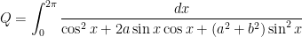

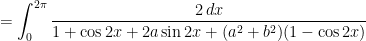
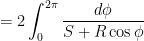
$Q = \displaystyle \int_0^{2\pi} \frac{dx}{\cos^2 x + 2 a \sin x \cos x + (a^2 + b^2) \sin^2 x}$

$= \displaystyle \int_0^{2\pi} \frac{2 \, dx}{1+\cos 2x + 2 a \sin 2x + (a^2 + b^2)(1-\cos 2x)}$

$= 2 \displaystyle \int_0^{2\pi} \frac{d\theta}{(1+a^2+b^2) + 2 a \sin \theta + (1 - a^2 - b^2) \cos \theta}$

$= 2 \displaystyle \int_{0}^{2\pi} \frac{d\theta}{S + R \cos (\theta - \alpha)}$

$= 2 \displaystyle \int_{0}^{2\pi} \frac{d\phi}{S + R \cos \phi}$

$= \displaystyle -\frac{4i}{R} \oint_C \frac{dz}{z^2 + 2\frac{S}{R}z + 1}$ ,

where this last integral is taken over the complex plane on the unit circle, a closed contour oriented counterclockwise. In these formulas, $R = \sqrt{(2a)^2 + (1-a^2-b^2)^2}$ and $S = 1 + a^2 + b^2$ . (Also, $\alpha$ is a certain angle that is now irrelevant at this point in the calculation).

This contour integral looks complicated; however, it’s an amazing fact that integrals over closed contours can be easily evaluated by only looking at the poles of the integrand. In recent posts, I established that there was only one pole inside the contour, and the residue at this pole was equal to $\displaystyle \frac{R}{ 2 \sqrt{S^2-R^2} }$ .

This residue can be used to evaluate the contour integral. Ordinarily, integrals are computed by subtracting the values of the antiderivative at the endpoints. However, there is an alternate way of computing a contour integral using residues. It turns out that the value of the contour integral is $2\pi i$ times the sum of the residues within the contour; see Wikipedia and Mathworld for more information.

Therefore,

$Q = \displaystyle -\frac{4i}{R} \oint_C \frac{dz}{(z - r_1)(z- r_2)}$

$= \displaystyle -\frac{4i}{R} \cdot 2\pi i \cdot \frac{R}{ 2 \sqrt{S^2-R^2} }$

$= \displaystyle \frac{4\pi}{\sqrt{S^2-R^2}}$

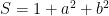
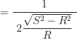
Next, I use some algebra to simplify the denominator:

$S^2 - R^2 = (1+a^2+b^2)^2 - (1-a^2-b^2)^2 - (2a)^2$

$S^2 - R^2 = [(1 + a^2 + b^2) + (1-a^2-b^2)][(1 + a^2 + b^2) - (1 - a^2 -b^2)] - 4a^2$

$S^2 - R^2 = 2[2 a^2 + 2b^2] - 4a^2$

$S^2 - R^2 = 4b^2$

Therefore,

$Q = \displaystyle \frac{4\pi}{\sqrt{4b^2}} = \displaystyle \frac{4\pi}{2|b|} = \frac{2\pi}{|b|}$

Once again, this matches the solution found with the previous methods… and I was careful to avoid a common algebraic mistake.

In tomorrow’s post, I’ll discuss an alternative way of computing the residue.

How I Impressed My Wife: Part 4e

Previously in this series, I have used two different techniques to show that

$Q = \displaystyle \int_0^{2\pi} \frac{dx}{\cos^2 x + 2 a \sin x \cos x + (a^2 + b^2) \sin^2 x} = \displaystyle \frac{2\pi}{|b|}.$

Here’s my progress so far:

$Q = \displaystyle \int_0^{2\pi} \frac{dx}{\cos^2 x + 2 a \sin x \cos x + (a^2 + b^2) \sin^2 x}$

$= \displaystyle \int_0^{2\pi} \frac{2 \, dx}{1+\cos 2x + 2 a \sin 2x + (a^2 + b^2)(1-\cos 2x)}$

$= 2 \displaystyle \int_0^{2\pi} \frac{d\theta}{(1+a^2+b^2) + 2 a \sin \theta + (1 - a^2 - b^2) \cos \theta}$

$= 2 \displaystyle \int_{0}^{2\pi} \frac{d\theta}{S + R \cos (\theta - \alpha)}$

$= 2 \displaystyle \int_{0}^{2\pi} \frac{d\phi}{S + R \cos \phi}$

$= \displaystyle -\frac{4i}{R} \oint_C \frac{dz}{z^2 + 2\frac{S}{R}z + 1}$

$= \displaystyle -\frac{4i}{R} \oint_C \frac{dz}{(z - r_1)(z- r_2)}$

where this last integral is taken over the complex plane on the unit circle, a closed contour oriented counterclockwise. Also,

$r_1 = \displaystyle \frac{-S + \sqrt{S^2 -R^2}}{R}$

and

$r_2 = \displaystyle \frac{-S - \sqrt{S^2 -R^2}}{R}$ ,

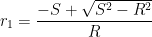
are the two distinct roots of the denominator (as long as $b \ne 0$ ). In these formulas, $R = \sqrt{(2a)^2 + (1-a^2-b^2)^2}$ and $S = 1 + a^2 + b^2$ . (Also, $\alpha$ is a certain angle that is now irrelevant at this point in the calculation).

This contour integral looks complicated; however, it’s an amazing fact that integrals over closed contours can be easily evaluated by only looking at the poles of the integrand. In yesterday’s post, I established that $r_1$ lies inside the contour, but $r_2$ lies outside of the contour.

The next step of the calculation is finding the residue at $r_1$ ; see Wikipedia and Mathworld for more information. This means rewriting the rational function

$\displaystyle \frac{1}{(z - r_1)(z - r_2)}$

as a power series (technically, a Laurent series) about the point $z = r_1$ . This can be done by using the formula for an infinite geometric series (see here, here, and here):

$\displaystyle \frac{1}{(z - r_1)(z - r_2)} = \displaystyle \frac{1}{z-r_1} \times \frac{1}{z-r_2}$

$= \displaystyle \frac{-1}{z-r_1} \times \frac{1}{r_2-z}$

$= \displaystyle \frac{-1}{z-r_1} \times \frac{1}{(r_2-r_1) - (z-r_1)}$

$= \displaystyle \frac{-1}{z-r_1} \times \frac{1}{r_2-r_1} \times \frac{ 1}{ 1 - \displaystyle \frac{z-r_1}{r_2-r_1} }$

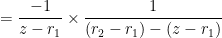
$= \displaystyle \frac{-1}{z-r_1} \times \frac{1}{r_2-r_1} \left[ 1 + \left( \displaystyle \frac{z-r_1}{r_2-r_1} \right) + \left( \displaystyle \frac{z-r_1}{r_2-r_1} \right)^2 + \left( \displaystyle \frac{z-r_1}{r_2-r_1} \right)^3 + \dots \right]$

$= \displaystyle \frac{-1}{z-r_1} \times \frac{1}{r_2-r_1} - \frac{1}{(r_2-r_1)^2} - \frac{z-r_1}{(r_2-r_1)^3} - \frac{(z-r_1)^2}{(r_2-r_1)^4} \dots$

The residue of the function at $z = r_1$ is defined to be the constant multiplying the $\displaystyle \frac{1}{z-r_1}$ term in the above series. Therefore,

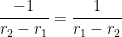
The residue at $x = r_1$ is $\displaystyle \frac{-1}{r_2-r_1} = \displaystyle \frac{1}{r_1-r_2}$

From the definitions of $r_1$ and $r_2$ above,

$\displaystyle \frac{1}{r_1-r_2} = \displaystyle \frac{1}{\displaystyle \frac{-S + \sqrt{S^2 -R^2}}{R} - \frac{-S - \sqrt{S^2 -R^2}}{R}}$

$= \displaystyle \frac{1}{ ~ 2 \displaystyle \frac{\sqrt{S^2-R^2}}{R} ~ }$

$= \displaystyle \frac{R}{ 2 \sqrt{S^2-R^2} }$

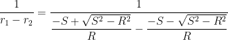
Now that I’ve identified the residue of the only root that lies inside of the contour, we are in position to evaluate the contour integral above. I’ll discuss this in tomorrow’s post.

Fun lecture on geometric series: Index

I’m using the Twelve Days of Christmas (and perhaps a few extra days besides) to do something that I should have done a long time ago: collect past series of posts into a single, easy-to-reference post. The following posts formed my series concerning one of my favorite lectures concerning various applications of geometric series.

Part 1: Introduction to generating functions.

Part 2: Enumeration problems; or counting how many ways $2.00 can be formed using pennies, nickels, dimes, and quarters. (The answer is 1463.)

Part 3: The generating function for the Fibonacci sequence.

Part 4: Using a generating function to find a closed-form expression for the (ahem) Quintanilla sequence, a close but somewhat less famous relative of the Fibonacci sequence.

Part 5: Reproving the formula for the Quintanilla sequence using mathematical induction.

Arithmetic and Geometric Series: Index

I’m using the Twelve Days of Christmas (and perhaps a few extra days besides) to do something that I should have done a long time ago: collect past series of posts into a single, easy-to-reference post. The following posts formed my series on how I remind students about Taylor series. I often use this series in a class like Differential Equations, when Taylor series are needed but my class has simply forgotten about what a Taylor series is and why it’s important.

Part 1: Deriving the formulas for the $n$ th term of arithmetic and geometric sequences.

Part 2: Pedagogical thoughts on conceptual barriers that students often face when encountering sequences and series.

Part 3: The story of how young Carl Frederich Gauss, at age 10, figured out how to add the integers from 1 to 100 in his head.

Part 4: Deriving the formula for an arithmetic series.

Part 5: Deriving the formula for an arithmetic series, using mathematical induction. Also, extensions to other series.

Part 6: Deriving the formula for an arithmetic series, using telescoping series. Also, extensions to other series.

Part 7: Pedagogical thoughts on assessing students’ depth of understanding the formula for an arithmetic series.

Part 8: Deriving the formula for a finite geometric series.

Part 9: Infinite geometric series and Xeno’s paradox.

Part 10: Deriving the formula for an infinite geometric series.

Part 11: Applications of infinite geometric series in future mathematics courses.

Part 12: Other commonly-arising infinite series.

2048 and algebra: Index

I’m doing something that I should have done a long time ago: collect past series of posts into a single, easy-to-reference post. The following posts formed my series on using algebra to study the 2048 game… with a special focus on reaching the event horizon of 2048 which cannot be surpassed.

2048-0 Part 1: Introduction and statement of problem

Part 2: First insight: How points are accumulated in 2048

Part 3: Second insight: The sum of the tiles on the board

Part 4: Algebraic formulation of the two insights

Part 5: Algebraic formulation applied to a more complicated board

Part 6: Algebraic formulation applied to the event horizon of 2048

Part 7: Calculating one of the complicated sums in Part 6 using a finite geometric series

Part 8: Calculating another complicated sum in Part 6 using a finite geometric series

Part 9: Repeating Part 8 by reversing the order of summation in a double sum

Part 10: Estimating the probability of reaching the event horizon in game mode

2048 and algebra (Part 9)

In this series of posts, I consider how algebra can be used to answer a question about the 2048 game: From looking at a screenshot of the final board, can I figure out how many moves were needed to reach the final board? Can I calculate how many new 2-tiles and 4-tiles were introduced to the board throughout the course of this game? In this post, we consider the event horizon of 2048, which I reached after about four weeks of intermittent doodling:

In yesterday’s post, we developed a system of two equations in two unknowns to solve for $t$ and $f$ , the number of 2-tiles and 4-tiles (respectively) that appeared throughout the course of the game:

$2t + 4f = \displaystyle \sum_{n=2}^{17} 2^n$ .

$2t + \displaystyle \sum_{n=1}^{15} n \cdot 2^{n+2} = 3,867,072$

In this post and tomorrow’s post, I consider how the two sums in the above equations can be obtained without directly adding the terms.

In yesterday’s post, we used the formula for the sum of a finite geometric series to calculate the second sum:

$\displaystyle \sum_{n=1}^{15} n \cdot 2^{n+2} = 14 \times 2^{18} + 2^3 = 3,670,024$

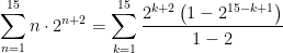
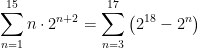
In this post, I perform this calculation again, except symbolically and more compactly. The key initial steps are writing the series as a double sum and then interchanging the order of summation (much like reversing the order of integration in a double integral). This is a trick that I’ve used again and again in my own research efforts, but it seems that the students that I teach have never learned this trick. Here we go:

$\displaystyle \sum_{n=1}^{15} n \cdot 2^{n+2} = \displaystyle \sum_{n=1}^{15} \sum_{k=1}^n 2^{n+2} = \displaystyle \sum_{k=1}^{15} \sum_{n=k}^{15} 2^{n+2}$

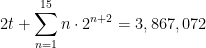
The inner sum is a finite geometric series with $15-k+1$ terms, common ratio of 2, and initial term $2^{k+2}$ . Therefore,

$\displaystyle \sum_{n=1}^{15} n \cdot 2^{n+2} = \displaystyle \sum_{k=1}^{15} \frac{ 2^{k+2} \left(1 - 2^{15-k+1} \right) }{1 - 2}$

$= \displaystyle \sum_{k=1}^{15} \left(2^{18} - 2^{k+2} \right)$

$= \displaystyle \sum_{k=1}^{15} 2^{18} -\sum_{k=1}^{15} 2^{k+2}$

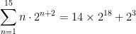
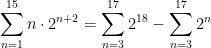
The first sum is merely the sum of a constant. The second sum is another finite geometric series with 15 terms, common ratio of 2, and initial term $2^3$ . So

$\displaystyle \sum_{n=1}^{15} n \cdot 2^{n+2} = 15 \times 2^{18} - \displaystyle \frac{ 2^3 \left(1 - 2^{15} \right) }{1 - 2}$

$\displaystyle \sum_{n=1}^{15} n \cdot 2^{n+2} = 15 \times 2^{18} - \left( 2^{18} - 2^3 \right)$

$\displaystyle \sum_{n=1}^{15} n \cdot 2^{n+2} = 14 \times 2^{18} + 2^3$

$\displaystyle \sum_{n=1}^{15} n \cdot 2^{n+2} = 3,670,024$

2048 and algebra (Part 8)

$2t + 4f = \displaystyle \sum_{n=2}^{17} 2^n$ .

$2t + \displaystyle \sum_{n=1}^{15} n \cdot 2^{n+2} = 3,867,072$

In this post and tomorrow’s post, I consider how the two sums in the above equations can be obtained without directly adding the terms.

In yesterday’s post, we showed that the formula for the sum of a finite geometric series can be used to calculate the first sum:

$\displaystyle \sum_{n=2}^{17} 2^n = \displaystyle \frac{4(1-2^{16})}{1-2} = 4(2^{15} - 1) = 262,140$

Let’s now consider the second (and more complicated) sum, which can be written as

$2^3 + 2 \cdot 2^4 + 3 \cdot 2^5 + \cdot + 15 \cdot 2^{17}$

For reasons that will become clear shortly, this sum can be written in expanded form as

$2^3$

$+ 2^4 + 2^4$

$+ 2^5 + 2^5 + 2^5$

$\vdots$

$+ 2^{17} + 2^{17} + 2^{17} + \dots + 2^{17}$

Let’s now rearrange the terms of this sum. We will do this by adding along the diagonals instead of along the rows. In this way, the above sum can be rearranged as

$2^3 + 2^4 + 2^5 + \dots + 2^{17}$

$+ 2^4 + 2^5 + \dots + 2^{17}$

$+ 2^5 + \dots + 2^{17}$

$\vdots$

$+ 2^{17}$

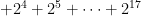
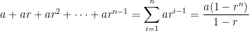
Each of these new rows (or the original diagonals) is a geometric series and can be calculated using the formula:

$2^3 + 2^4 + 2^5 + \dots + 2^{17} = \displaystyle \frac{2^3 (1-2^{15})}{1-2} = 2^{18} - 2^3$

$2^4 + 2^5 + \dots + 2^{17} = \displaystyle \frac{2^4 (1-2^{14})}{1-2} = 2^{18} - 2^4$

$2^5 + \dots + 2^{17} = \displaystyle \frac{2^5 (1-2^{13})}{1-2} = 2^{18} - 2^5$

$\vdots$

$2^{17} = (2-1) \cdot 2^{17} = 2^{18} - 2^{17}$

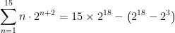
So, thus far in the calculation, we have established that

$\displaystyle \sum_{n=1}^{15} n \cdot 2^{n+2} = \displaystyle \sum_{n=3}^{17} \left( 2^{18} - 2^n \right)$ .

Simplifying,

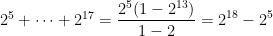
$\displaystyle \sum_{n=1}^{15} n \cdot 2^{n+2}=\displaystyle \sum_{n=3}^{17} 2^{18} - \sum_{n=3}^{17} 2^n$

The first sum on the right is the sum of a constant being added to itself 15 times:

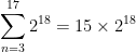
$\displaystyle \sum_{n=3}^{17} 2^{18} = 15 \times 2^{18}$

The second sum on the right is yet another geometric series. Indeed, it’s the same geometric series from the first diagonal above:

$\sum_{n=3}^{17} 2^n = \displaystyle \frac{2^3 (1-2^{15})}{1-2} = 2^{18} - 2^3$

Therefore,

$\displaystyle \sum_{n=1}^{15} n \cdot 2^{n+2} = 15 \times 2^{18} - \left(2^{18} - 2^3 \right)$

$\displaystyle \sum_{n=1}^{15} n \cdot 2^{n+2} = 14 \times 2^{18} + 2^3$

$\displaystyle \sum_{n=1}^{15} n \cdot 2^{n+2} = 3,670,024$

Not surprisingly, this matches the sum that was found via direct addition.

2048 and algebra (Part 7)

$2t + 4f = \displaystyle \sum_{n=2}^{17} 2^n$ .

$2t + \displaystyle \sum_{n=1}^{15} n \cdot 2^{n+2} = 3,867,072$

In this post and tomorrow’s post, I consider how the two sums in the above equations can be obtained without directly adding the terms.

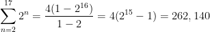
The first sum is certainly the easiest to handle, as it requires the sum of a finite geometric series:

$a + ar + ar^2 + \dots + a r^{n-1} = \displaystyle \sum_{i=1}^n a r^{i-1} = \displaystyle \frac{a(1-r^n)}{1-r}$

For the geometric series

$\displaystyle \sum_{n=2}^{17} 2^n$ ,

there are 16 terms (after all, there are 16 tiles on the board). The first term is 4, and the common ratio is 2. Therefore,

$\displaystyle \sum_{n=2}^{17} 2^n = \displaystyle \frac{4(1-2^{16})}{1-2}$

$\displaystyle \sum_{n=2}^{17} 2^n = 4(2^{15} - 1)$

$\displaystyle \sum_{n=2}^{17} 2^n = 262,140$

We’ll consider the more complicated sum in tomorrow’s post.

Exponential growth and decay (Part 6): Paying off credit-card debt via recurrence relations

The following problem in differential equations has a very practical application for anyone who has either (1) taken out a loan to buy a house or a car or (2) is trying to pay off credit card debt. To my surprise, most math majors haven’t thought through the obvious applications of exponential functions as a means of engaging their future students, even though it is directly pertinent to their lives (both the students’ and the teachers’).

You have a balance of $2,000 on your credit card. Interest is compounded continuously with a rate of growth of 25% per year. If you pay the minimum amount of $50 per month (or $600 per year), how long will it take for the balance to be paid?

In previous posts, I approached this problem using differential equations. There’s another way to approach this problem that avoids using calculus that, hypothetically, is within the grasp of talented Precalculus students. Instead of treating this problem as a differential equation, we instead treat it as a first-order difference equation (also called a recurrence relation):

$A_{n+1} = r A_n - k$

The idea is that the amount owed is multiplied by a factor $r$ (which is greater than 1), and from this product the amount paid is deducted. With this approach — and unlike the approach using calculus — the payment period would be each month and not per year. Therefore, we can write

$A_{n+1} = \displaystyle \left( 1 + \frac{0.25}{12} \right) A_n - 50$

Notice that the meaning of the 25% has changed somewhat… it’s no longer the relative rate of growth, as the 25% has been equally divided for the 12 months.

green line

In yesterday’s post, I demonstrated that the solution of this recurrence relation is

$A_n = r^n P - k \displaystyle \left( \frac{1 - r^n}{1-r} \right)$ .

Let’s now study when the credit card debt will actually reach $0. To do this, we see $A_n = 0$ and solve for $n$ :

$0 = r^n P - k \displaystyle \left( \frac{1 - r^n}{1-r} \right)$

$0 = r^n \left(P + \displaystyle \frac{k}{1-r} \right) - \displaystyle \frac{k}{1-r}$

$0 = r^n \left( P[1-r] + k \right) - k$

$k = r^n \left( P[1-r] + k \right)$

$\displaystyle \frac{k}{P[1-r] + k} = r^n$

$\displaystyle \ln \left( \frac{k}{P[1-r]+k} \right) = n \ln r$

$\displaystyle \frac{ \displaystyle \ln \left( \frac{k}{P[1-r]+k} \right) }{ \ln r} = n$

That’s certainly a mouthful. However, this calculation should be accessible to a talented student in Precalculus.

Let’s try it out for $k = 50$ , $P = 2000$ , and $r = 1 + \displaystyle \frac{0.25}{12}$ :

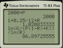
Remembering that each compounding period is one month long, this corresponds to $86.897/12 \approx 7.24$ years, which is nearly equal to the value of $4\ln 6 \approx 7.17$ years when we solved this problem using differential equations under the assumption of continuous compound interest (as opposed to interest that’s compoounded monthly).

Tag: geometric series

Zeno’s Hairodox

How I Impressed My Wife: Part 4f

How I Impressed My Wife: Part 4e

Fun lecture on geometric series: Index

Arithmetic and Geometric Series: Index

2048 and algebra: Index

2048 and algebra (Part 9)

2048 and algebra (Part 8)

2048 and algebra (Part 7)

Exponential growth and decay (Part 6): Paying off credit-card debt via recurrence relations