At long last, we have reached the end of this series of posts.
The derivation is elementary; I’m confident that I could have understood this derivation had I seen it when I was in high school. That said, the word “elementary” in mathematics can be a bit loaded — this means that it is based on simple ideas that are perhaps used in a profound and surprising way. Perhaps my favorite quote along these lines was this understated gem from the book Three Pearls of Number Theory after the conclusion of a very complicated proof in Chapter 1:
You see how complicated an entirely elementary construction can sometimes be. And yet this is not an extreme case; in the next chapter you will encounter just as elementary a construction which is considerably more complicated.
Here are the elementary ideas from calculus, precalculus, and high school physics that were used in this series:
- Physics
- Conservation of angular momentum
- Newton’s Second Law
- Newton’s Law of Gravitation
- Precalculus
- Completing the square
- Quadratic formula
- Factoring polynomials
- Complex roots of polynomials
- Bounds on
and
- Period of
- Zeroes of
- Trigonometric identities (Pythagorean, sum and difference, double-angle)
- Conic sections
- Graphing in polar coordinates
- Two-dimensional vectors
- Dot products of two-dimensional vectors (especially perpendicular vectors)
- Euler’s equation
- Calculus
- The Chain Rule
- Derivatives of
- Linearizations of
,
, and
near
(or, more generally, their Taylor series approximations)
- Derivative of
- Solving initial-value problems
- Integration by
substitution


While these ideas from calculus are elementary, they were certainly used in clever and unusual ways throughout the derivation.
I should add that although the derivation was elementary, certain parts of the derivation could be made easier by appealing to standard concepts from differential equations.
One more thought. While this series of post was inspired by a calculation that appeared in an undergraduate physics textbook, I had thought that this series might be worthy of publication in a mathematical journal as an historical example of an important problem that can be solved by elementary tools. Unfortunately for me, Hieu D. Nguyen’s terrific article Rearing Its Ugly Head: The Cosmological Constant and Newton’s Greatest Blunder in The American Mathematical Monthly is already in the record.

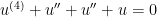
 th order homogeneous differential equation with constant coefficients
 ,
,
 determines the solutions of the differential equation.
 . Differentiating, we find
  ,
,  , etc. Therefore, the differential equation becomes


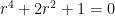
 can never be equal to
  . Therefore, solving the differential equation reduces to finding the roots of this polynomial, which can be done using standard techniques from Precalculus.
 . The characteristic equation is
  , which has roots
  . Therefore, two solutions to the differential equation are
  and
and  , so that the general solution is
 .
. , so that


 .
. . To find the roots of the characteristic equation, we factor:


 .
. , and
, and  , so that the general solution is
 .
. .
. with the Sun at the origin, under general relativity follows the initial-value problem
  ,
, ,
, ,
, ,
,  ,
,  ,
,  is the gravitational constant of the universe,
  is the mass of the planet,
  is the mass of the Sun,
  is the constant angular momentum of the planet,
  is the speed of light, and
  is the smallest distance of the planet from the Sun during its orbit (i.e., at perihelion).
  .
. .
. .
. . Then
  satisfies the new differential equation
  . Also,
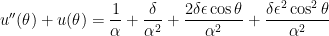
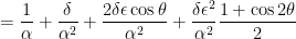
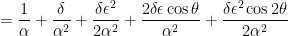
  . Substituting, we find


 .
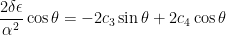
. and
and  can be found by substituting back into the original differential equation:

 and
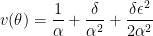
and  . Therefore, the solution of the simplified differential equation is
 .
. and
and  , we see that

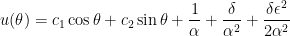
 is some unknown function, to find the general solution of the differential equation
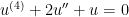 .
.
 .
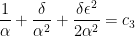
. . If
. If  , then
 ,
, ,
, ,
, .
.


 and
and  cancelled each other. This new differential equation doesn’t look like much of an improvement over the original fourth-order differential equation, but we can make a key observation: if
  , then differentiating twice more trivially yields
  and
and  . Said another way: if

 .
. .
. :
:


 .
. , so that
  . Therefore, another solution of the original differential equation will be
 .
. .
. .
. ,
, .
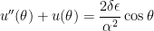
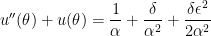
. , which corresponds to the second-order differential equation
  . We’ve already seen that
  and
and  are solutions of this differential equation; perhaps they might also be solutions of the more complicated differential equation also? The answer, of course, is yes:
 .
. ,
, .
. :
:![(fg)'' = ( [fg]')' = (f'g)' + (fg')'](https://s0.wp.com/latex.php?latex=%28fg%29%27%27+%3D+%28+%5Bfg%5D%27%29%27+%3D+%28f%27g%29%27+%2B+%28fg%27%29%27&bg=ffffff&fg=000000&s=0&c=20201002)

 .
. :
:![(fg)''' = ( [fg]'')' = (f''g)' + 2(f'g')' + (fg'')'](https://s0.wp.com/latex.php?latex=%28fg%29%27%27%27+%3D+%28+%5Bfg%5D%27%27%29%27+%3D+%28f%27%27g%29%27+%2B+2%28f%27g%27%29%27+%2B++%28fg%27%27%29%27&bg=ffffff&fg=000000&s=0&c=20201002)

 .
.![(fg)^{(4)} = ( [fg]''')' = (f'''g)' + 3(f''g')' +3(f'g'')' + (fg''')'](https://s0.wp.com/latex.php?latex=%28fg%29%5E%7B%284%29%7D+%3D+%28+%5Bfg%5D%27%27%27%29%27+%3D+%28f%27%27%27g%29%27+%2B+3%28f%27%27g%27%29%27+%2B3%28f%27g%27%27%29%27+%2B+%28fg%27%27%27%29%27&bg=ffffff&fg=000000&s=0&c=20201002)

 .
. .
. . Then
  . Since
  , we may substitute:
 . Therefore,
  and
and  are both double roots of this quartic equation. Therefore, the general solution for
  is
is .
.

 and
and  . Therefore,
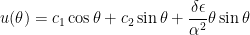
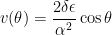
 , we find that
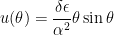
 term is what predicts the precession of a planet’s orbit under general relativity.
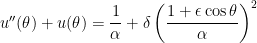 ,
,
 .
. . Since
  . Since
  , we can substitute:

 . Factoring, we obtain
  , so that the three roots are
  and
and  . Therefore, the general solution of this differential equation is
 .
. and
and  are determined by the initial conditions. To find
 .
. .
.
 .
.


