In this series of posts, I explore properties of complex numbers that explain some surprising answers to exponential and logarithmic problems using a calculator (see video at the bottom of this post). These posts form the basis for a sequence of lectures given to my future secondary teachers.
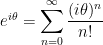
Definition. If  is a complex number, then we define

Even though this isn’t the usual way of defining the exponential function for real numbers, the good news is that one Law of Exponents remains true. (At we saw in an earlier post in this series, we can’t always assume that the usual Laws of Exponents will remain true when we permit the use of complex numbers.)
Theorem. If and  are complex numbers, then
  .
.
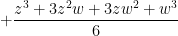
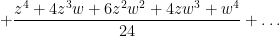
In yesterday’s post, I gave the idea behind the proof… group terms where the sums of the exponents of and are the same. Today, I will formally prove the theorem.
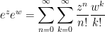
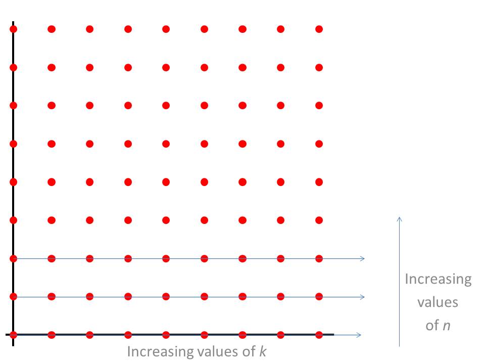
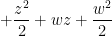
The proof of the theorem relies on a principle that doesn’t seem to be taught very often anymore… rearranging the terms of a double sum. In this case, the double sum is
This can be visualized in the picture below, where the  axis represents the values of
  and the
  axis represents the values of
  . Each red dot symbolizes a term in the above double sum. For a fixed value of , the values of vary from
  to
to  . In other words, we start with
  and add all the terms on the line
  (i.e., the axis in the picture). Then we go up to
  and then add all the terms on the next horizontal line. And so on.

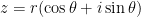
I will rearrange the terms as follows: Let  . Then for a fixed value of
  , the values of will vary from to . This is perhaps best described in the picture below. The value of , the sum of the coordinates, is constant along the diagonal lines below. The value of then changes while moving along a diagonal line.
Even though this is a different way of adding the terms, we clearly see that all of the red circles will be hit regardless of which technique is used for adding the terms.

In this way, the double sum  gets replaced by
  . Since
  , we have

We now add a couple of  terms to this expression for reasons that will become clear shortly:

Since does not contain any s, it can be pulled outside of the inner sum on . We do this for the in the denominator:

We recognize that  is a binomial coefficent:
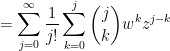
The inner sum is recognized as the formula for a binomial expansion:

Finally, we recognize this as the definition of  , using the dummy variable instead of . This proves that even if and are complex.
Without a doubt, this theorem was a lot of work. The good news is that, with this result, it will no longer be necessary to explicitly use the summation definition of  to actually compute , as we’ll see tomorrow.
 For completeness, here’s the movie that I use to engage my students when I begin this sequence of lectures.


![= e^{-\pi} (\cos [\ln 8] + i \sin [ \ln 8 ] )](https://s0.wp.com/latex.php?latex=%3D+e%5E%7B-%5Cpi%7D+%28%5Ccos+%5B%5Cln+8%5D+%2B+i+%5Csin+%5B+%5Cln+8+%5D+%29&bg=ffffff&fg=000000&s=0&c=20201002)


 . However, this complex logarithm doesn’t always work the way you’d think it work. For example,
 .
.
 .
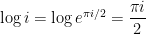
.![\log \left[ (-1) \cdot (-1) \right] = \log 1 = 0](https://s0.wp.com/latex.php?latex=%5Clog+%5Cleft%5B+%28-1%29+%5Ccdot+%28-1%29+%5Cright%5D+%3D+%5Clog+1+%3D+0&bg=ffffff&fg=000000&s=0&c=20201002) ,
, .
. ,
, .
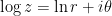
.![(-\pi,\pi]](https://s0.wp.com/latex.php?latex=%28-%5Cpi%2C%5Cpi%5D&bg=ffffff&fg=000000&s=0&c=20201002) leads to the definition of the complex logarithm.
leads to the definition of the complex logarithm.
 .
. is usually dedicated to base 10. However, in higher-level mathematics courses,
  , but
, but  requires a little more thought. But nearly all major theorems that involve logarithms specifically employ natural logarithms. Indeed, when I first become a professor, I had to remind myself that my students used
  for natural logarithms and not
  for base-10 logarithms and not
  is entered, it assumes that a real answer is expected, and so the calculatore returns an error message. On the other hand, when
  is entered, it assumes that the user wants the principal complex logarithm. Since
  , the calculator correctly returns
  as the answer. (Of course, the calculator still uses
  .
. , then
 and that the angle
  and
and  for any integer
  .
. . This could have been any nonzero number, including complex numbers, and there still would have been an infinite number of solutions. (This is completely analogous to solving a trigonometric equation like
  , which similarly has an infinite number of solutions.) For example, the complex solutions of the equation
 is
is  .
. .
. for real numbers
  .
.
 to a power and get a negative number. Obviously, this is impossible when using only real numbers.

 to represent
  . I say this because I’ve seen textbooks that basically invented the non-standard notation
  (pronounced siss), where presumably the c represents
  and the s represents
  . I express my contempt for this non-standard notation by saying that this is a sissy way of writing it.
![\left[ r_1 ( \cos \theta_1 + i \sin \theta_1) \right] \cdot \left[ r_2 ( \cos \theta_2 + i \sin \theta_2 ) \right] = r_1 r_2 \left[ \cos( \theta_1 + \theta_2) + i \sin (\theta_1 + \theta_2) \right]](https://s0.wp.com/latex.php?latex=%5Cleft%5B+r_1+%28+%5Ccos+%5Ctheta_1+%2B+i+%5Csin+%5Ctheta_1%29+%5Cright%5D+%5Ccdot+%5Cleft%5B+r_2+%28+%5Ccos+%5Ctheta_2+%2B+i+%5Csin+%5Ctheta_2+%29+%5Cright%5D+%3D+r_1+r_2+%5Cleft%5B+%5Ccos%28+%5Ctheta_1+%2B+%5Ctheta_2%29+%2B+i+%5Csin+%28%5Ctheta_1+%2B+%5Ctheta_2%29+%5Cright%5D&bg=ffffff&fg=000000&s=0&c=20201002)

![\displaystyle \frac{ r_1 ( \cos \theta_1 + i \sin \theta_1)}{ r_2 ( \cos \theta_2 + i \sin \theta_2 ) } = \displaystyle \frac{r_1}{ r_2} \left[ \cos( \theta_1 - \theta_2) + i \sin (\theta_1 - \theta_2) \right]](https://s0.wp.com/latex.php?latex=%5Cdisplaystyle+%5Cfrac%7B+r_1+%28+%5Ccos+%5Ctheta_1+%2B+i+%5Csin+%5Ctheta_1%29%7D%7B+r_2+%28+%5Ccos+%5Ctheta_2+%2B+i+%5Csin+%5Ctheta_2+%29+%7D+%3D+%5Cdisplaystyle+%5Cfrac%7Br_1%7D%7B+r_2%7D+%5Cleft%5B+%5Ccos%28+%5Ctheta_1+-+%5Ctheta_2%29+%2B+i+%5Csin+%28%5Ctheta_1+-+%5Ctheta_2%29+%5Cright%5D&bg=ffffff&fg=000000&s=0&c=20201002)

![\left[ r (\cos \theta + i \sin \theta) \right]^n = r^n (\cos n \theta + i \sin n \theta)](https://s0.wp.com/latex.php?latex=%5Cleft%5B+r+%28%5Ccos+%5Ctheta+%2B+i+%5Csin+%5Ctheta%29+%5Cright%5D%5En+%3D+r%5En+%28%5Ccos+n+%5Ctheta+%2B+i+%5Csin+n+%5Ctheta%29&bg=ffffff&fg=000000&s=0&c=20201002)

 .
.

 ,
, .
. would be next to impossible by directly plugging into the series and trying to simply the answer. The good news is that there’s an easy way to compute


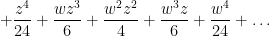
 ,
,  ,
,  , and
, and  are placed together because the sum of the exponents for each of these terms is 3.


 ,
, which is demonstrated in the video below.