Sadly, at least at my university, Taylor series is the topic that is least retained by students years after taking Calculus II. They can remember the rules for integration and differentiation, but their command of Taylor series seems to slip through the cracks. In my opinion, the reason for this lack of retention is completely understandable from a student’s perspective: Taylor series is usually the last topic covered in a semester, and so students learn them quickly for the final and quickly forget about them as soon as the final is over.
Of course, when I need to use Taylor series in an advanced course but my students have completely forgotten this prerequisite knowledge, I have to get them up to speed as soon as possible. Here’s the sequence that I use to accomplish this task. Covering this sequence usually takes me about 30 minutes of class time.
I should emphasize that I present this sequence in an inquiry-based format: I ask leading questions of my students so that the answers of my students are driving the lecture. In other words, I don’t ask my students to simply take dictation. It’s a little hard to describe a question-and-answer format in a blog, but I’ll attempt to do this below.
In the previous posts, I described how I lead students to the definition of the Maclaurin series
 ,
,
which converges to  within some radius of convergence for all functions that commonly appear in the secondary mathematics curriculum.

Step 5. That was easy; let’s try another one. Now let’s try 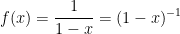 .
.
What’s  ? Plugging in, we find
  .
.
Next, to find  , we first find
  . Using the Chain Rule, we find
 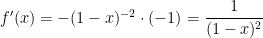 , so that
  .
.
Next, we differentiate again:  , so that
  .
.
Hmmm… no obvious pattern yet… so let’s keep going.
For the next term, 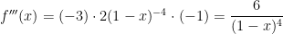 , so that
  .
.
For the next term,  , so that
  .
.
Oohh… it’s the factorials again! It looks like  , and this can be formally proved by induction.
Plugging into the series, we find that
 .
.
Like the series for  , this series converges quickest for
  . Unlike the series for , this series does not converge for all real numbers. As can be checked with the Ratio Test, this series only converges if
  .
.
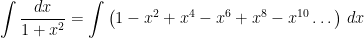
The right-hand side is a special kind of series typically discussed in precalculus. (Students often pause at this point, because most of them have forgotten this too.) It is an infinite geometric series whose first term is $1$ and common ratio $x$. So starting from the right-hand side, one can obtain the left-hand side using the formula

by letting  and $r=x$. Also, as stated in precalculus, this series only converges if the common ratio satisfies $|r| < 1$, as before.
In other words, in precalculus, we start with the geometric series and end with the function. With Taylor series, we start with the function and end with the series.
Step 6. A whole bunch of other Taylor series can be quickly obtained from the one for  . Let’s take the derivative of both sides (and ignore the fact that one should prove that differentiating this infinite series term by term is permissible). Since

and
 ,
,
we have
 .
.
____________________
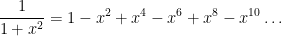
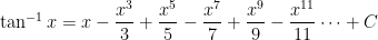
Next, let’s replace  with
with  in the Taylor series in Step 5, obtaining

Now let’s take the indefinite integral of both sides:


To solve for the constant of integration, let  :
:

Plugging back in, we conclude that

The Taylor series expansion for  can be found by replacing with :

Subtracting, we find

My understanding is that this latter series is used by calculators when computing logarithms.
____________________
Next, let’s replace with  in the Taylor series in Step 5, obtaining
Now let’s take the indefinite integral of both sides:
To solve for the constant of integration, let :

Plugging back in, we conclude that

____________________
In summary, a whole bunch of Taylor series can be extracted quite quickly by differentiating and integrating from a simple infinite geometric series. I’m a firm believer in minimizing the number of formulas that I should memorize. Any time I personally need any of the above series, I’ll quickly use the above steps to derive them from that of .


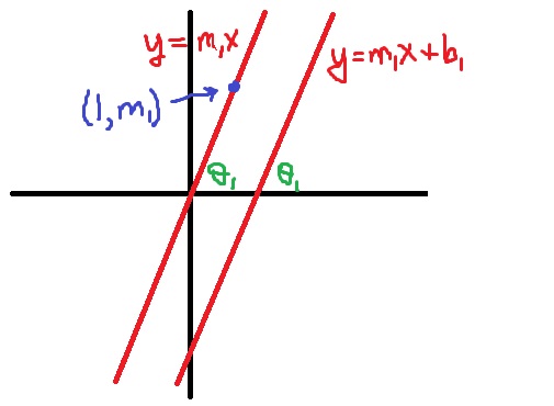 The lines


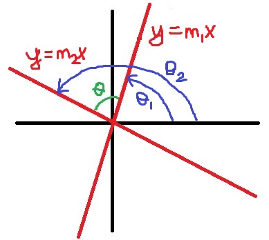


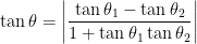


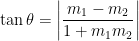


 and
and  .
.
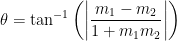
 and
and  . I use the caveat almost because the angle between two vectors could be between
  , while the smallest angle between two lines must lie between
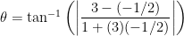


 .
. .
.
 :
:
 , we select a section that satisfies the horizontal line test and ignore the rest of the graph. (I described this in more rigorous terms when I considered arcsine, so I will not repeat the rigor here.) There are plenty of choices that could be made; by tradition, the interval
 ![[0,\pi]](https://s0.wp.com/latex.php?latex=%5B0%2C%5Cpi%5D&bg=ffffff&fg=000000&s=0&c=20201002) is chosen.
is chosen.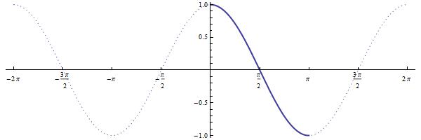
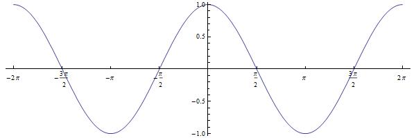
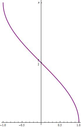
 produces the graph of
  . Again, to assist my students when graphing this function, I point out that the graph of cosine has horizontal tangent lines at the points
  and
and  . Therefore, after reflecting through the line
  has vertical tangent lines at
  and
and  .
.
 is chosen as the section of the graph of
  that satisfies the horizontal line test.
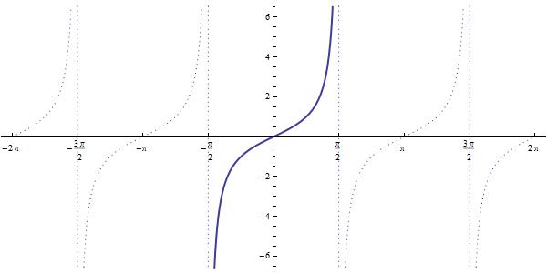
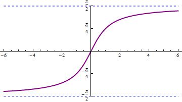
 . Like the (more complicated)
  .
.
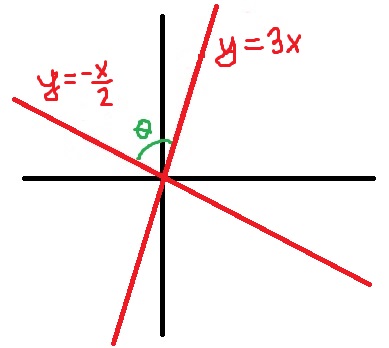
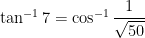
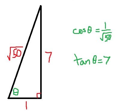
 means that
  and
and 
 means that
  and
and 


 . I told the class that I had worked this out ahead of time, and that the approximate answer was
  . Then I used that angle for whatever I needed it for and continued until obtaining the eventual solution.
 ?
? , thanks to my calculation prior to class. I also knew that
  since the graph of
  . So the solution to
  had to be somewhere between
  .
. ,” I said, faking complete and utter confidence.
 .)
.)