In my capstone class for future secondary math teachers, I ask my students to come up with ideas for engaging their students with different topics in the secondary mathematics curriculum. In other words, the point of the assignment was not to devise a full-blown lesson plan on this topic. Instead, I asked my students to think about three different ways of getting their students interested in the topic in the first place.
I plan to share some of the best of these ideas on this blog (after asking my students’ permission, of course).
This student submission again comes from my former student Randall Hall. His topic, from Geometry: defining the terms acute, right, and obtuse.

D4. What are the contributions of various cultures to this topic?
In ancient times, Euclid adopted the idea of a right angle and defined a right angle to be an angle that was to be congruent to it, an acute angle was denoted by less than a right angle and obtuse angle was denoted to be greater than a right angle. Euclid defined it that way because back then Geometry wasn’t associated with numbers; Geometry was associated with circles, lines, line segments and triangles. Many things we know now such as the Pythagorean Theorem can be explained by what we know now to be a right angle.
The Babylonians were one of the first to use degrees in measurements of astronomy between 5000 and 4000 BC. The Babylonians had an interesting number system in that they used a base-60 counting system while today we use a base-10 system. It is because of them that we have a sixty minutes in an hour and 360 degrees in a circle.
Source: http://math.ucsd.edu/~wgarner/math4c/textbook/chapter5/angles_radians.htm
D5. How have different cultures throughout time used this topic in their society?
The history of the mathematical measurement of angles possibly dates back to 1500BC in Egypt, where measurements were taken of the Sun’s shadow against graduations marked on stone tables, examples of which can be seen in the Egyptian Museum in Berlin. The shadow was cast but a vertical rod (Gnomon) along the length of the markings on a stone tablet, enabling time and seasons to be measured with some degree of accuracy.
The first known instrument for measuring angles was possibly the Egyptian Groma, an instrument used in construction massive objects such as the pyramids. The Groma consisted of four stones hanging by cords from sticks set at right angles; measurements were then taken by the visual alignment of two of the suspended cords and the point to be set out. It was limited due to it was only usable on fairly flat terrain and its accuracy limited by distance. The Groma continued to set out right angles for many Roman constructions, including roads, which were straight lines, set by the Groma.
Source: http://www.fig.net/pub/cairo/papers/wshs_01/wshs01_02_wallis.pdf
E1. How can technology (YouTube, Khan Academy [khanacademy.org], Vi Hart, Geometers Sketchpad, graphing calculators, etc.) be used to effectively engage students with this topic?
The link below contains a great JAVA applet that features an angle within the apple that allows the user to designate what the user wants the angle to be. In addition to showing the angle, the applet will recognize that number and then output the appropriate angle type. For example, if the applet recognizes a 90 in the “degree of angle” box and then outputs ‘Right’. In addition to the JAVA application, a description of an angle is given for each type of angle. The classifications of angles are: acute, right, obtuse, straight, reflux, and full rotation. This is excellent for the student because it provides the student a visual of what each type of angles look like. Visuals, such as this, are good for the student because it encompasses all types of learning style. It is also good for ESL learners because it provides them an alternative method for interpreting what is being discussed.
http://www.cut-the-knot.org/Curriculum/Geometry/Angle.shtml


 Using this, the main theorem follows by using diagonals to divide a convex n-gon into


 and
and  can be found using the formula
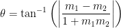 .
. and
and  axis.
axis.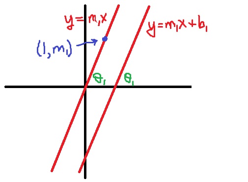
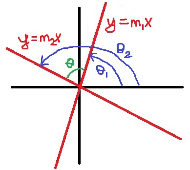
 is entirely superfluous to finding the angle
  . The important thing that matters is the slope of the line, not where the line intersects the
  axis.
axis. lies on the line
  can be found by dividing the
  .
.
 .
. will either be equal to
  or
or  , depending on the values of
  and
and  . Let’s now compute both
  and
and  using the formula for the difference of two angles:

 and
and  , the value of
  must be positive (or undefined if
  … for now, we’ll ignore this special case). Therefore, whichever of the above two lines holds, it must be that
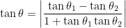
 and
and  :
:

 , and the right hand side is also undefined if
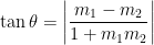
  . This matches the theorem that the two lines are perpendicular if and only if
  , or that the slopes of the two lines are negative reciprocals.
 and
and  .
.
 and
and  . I use the caveat almost because the angle between two vectors could be between
  , while the smallest angle between two lines must lie between
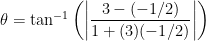


 .
. .
.
 and
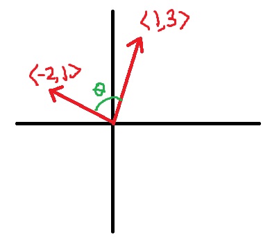
and  . To begin, we draw the vectors
  (to be determined momentarily) that connects the tips of the vectors
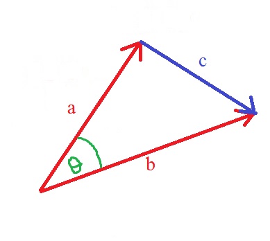
 , so that


 , convert the square of the norms into dot products. We then use the distributive and commutative properties of dot products to simplify.


 :
:
 and
and  ). Since this is the range of arccosine, we are permitted to use this inverse function to solve for
 for any dimension
  .
.
 and
and 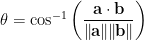
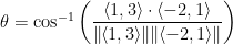
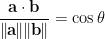
 is the dot product (or inner product) of the two vectors
  is the norm (or length) of the vector