A probability problem involving two cards (Part 3)

In yesterday’s post, I gave two solutions that a student gave to the following probability problem. One of the solutions was correct, and one of the solutions was incorrect.

Two cards are dealt from a well-shuffled deck. Find the probability that the first is an ace or the second is a jack.

What follows is the incorrect (but, as we’ll see later, salvageable) solution.

Method #2 (incorrect):There are three ways that either the first or second card could be an a jack:

The first card is an ace and the second card is a jack.
The first card is an ace and the second card is not a jack.
The first card is not an ace and the second card is a jack.

Each of these can be computed using the rule $P(A \cap B) = P(A) P(B \mid A)$ in much the same way as above:

P(first an ace) P(second a jack, given first an ace) $= \displaystyle \frac{4}{52} \cdot \frac{4}{51}$
P(first an ace) P(second not a jack, given first an ace) $= \displaystyle \frac{4}{52} \cdot \frac{47}{51}$
P(first not an ace) P(second a jack, given first not an ace) $= \displaystyle \frac{48}{52} \cdot \frac{4}{51}$

Adding these together, we obtain the answer:

$\displaystyle \frac{4}{52} \cdot \frac{4}{51} + \frac{4}{52} \cdot \frac{47}{51} + \frac{48}{52} \cdot \frac{4}{51}$

$= \displaystyle \frac{4 \times 4 + 4 \times 47 + 48 \times 4}{52 \times 51}$

$= \displaystyle \frac{4 + 47 + 48}{13 \times 51}$

$= \displaystyle \frac{99}{663}$

When my student presented this to me, I must admit that it took me a couple of minutes before I found the hole in the student’s logic.

This answer is wrong because the second probability in Case 3 above was not calculated correctly. If we only know that the first card is not an ace, then we don’t have enough information to know how many of the remaining 51 cards are jacks. So the conditional probability $\displaystyle \frac{4}{51}$ is incorrect in Step 3.

Even though the above logic is slightly incorrect, it can be salvaged by splitting Case 3 above into two subcases.

Method #2:There are three ways that either the first or second card could be an a jack:

The first card is an ace and the second card is a jack.
The first card is an ace and the second card is not a jack.
The first card is a jack, and the second card is a jack.
The first card is neither an ace nor a jack, and the second card is a jack.

Each of these can be computed using the rule $P(A \cap B) = P(A) P(B \mid A)$ :

P(first an ace) P(second a jack, given first an ace) $= \displaystyle \frac{4}{52} \cdot \frac{4}{51}$
P(first an ace) P(second not a jack, given first an ace) $= \displaystyle \frac{4}{52} \cdot \frac{47}{51}$
P(first a jack) P(second a jack, given first a jack) $= \displaystyle \frac{4}{52} \cdot \frac{3}{51}$
P(first neither an ace or a jack) P(second a jack, given first neither an ace or a jack) $= \displaystyle \frac{44}{52} \cdot \frac{4}{51}$

By splitting the original Case 3 into the new Cases 3 and 4, there is no longer any ambiguity about how many jacks remain when the second card is chosen. Adding these together, we obtain the answer:

$\displaystyle \frac{4}{52} \cdot \frac{4}{51} + \frac{4}{52} \cdot \frac{47}{51} + \frac{4}{52} \frac{3}{51} + \frac{44}{52} \cdot \frac{4}{51}$

$= \displaystyle \frac{4 \times 4 + 4 \times 47 + 4 \times 3 + 44 \times 4}{52 \times 51}$

$= \displaystyle \frac{4 + 47 + 3 + 44}{13 \times 51}$

$= \displaystyle \frac{98}{663}$

Not surprisingly, this matches the answer obtained when the formula $P(A \cup B) = P(A) + P(B) - P(A \cap B)$ was employed in yesterday’s post.

A probability problem involving two cards (Part 2)

Here is a standard problem that could appear in an elementary probability class.

Two cards are dealt from a well-shuffled deck. Find the probability that the first is an ace or the second is a jack.

In yesterday’s post, I considered two different ways of solving a similar-looking problem, except the final word jack was replaced by ace. Yesterday, I showed that there were two legitimate ways of solving that problem, resulting (of course) in the same answer.

About a year ago, a student came into my office using these two different techniques to solve the ace/jack problem. Except she arrived at two different answers!

Method #1: One law for probability states that

$P(A \cup B) = P(A) + P(B) - P(A \cap B)$

Another law of probability states that

$P(A \cap B) = P(A) P(B \mid A)$

Combining these, we find that

$P(A \cup B) = P(A) + P(B) - P(A) P(B \mid A)$

Written more colloquially,

P(first an ace or second a jack)

= P(first an ace) + P(second a jack) – P(first an ace AND second a jack)

=P(first an ace) + P(second a jack) – P(first an ace) P(second a jack, given first an ace)

Let’s look at these three probabilities on the last line separately.

P(first an ace) is $\displaystyle \frac{4}{52}$ .
P(second a jack) is also $\displaystyle \frac{4}{52}$ . No information about the first card appears between the two parentheses, and so this is similar to pulling a card out of the middle of a deck. Since no information is given about the preceding card(s), the answer is still $\displaystyle \frac{4}{52}$ .
P(second an a jack, given first an ace) is different than the answer to #2 above. For this problem, the first card is known to be an ace, and the question is, given this knowledge, what is the probability that the second card is a jack? Since the first card is known to be an ace, there are still 4 jacks left out of 51 possible cards. Therefore, the answer is $\displaystyle \frac{4}{51}$ .

Putting these together, we find the final solution of

$\displaystyle \frac{4}{52} + \frac{4}{52} - \frac{4}{52} \cdot \frac{4}{51}$

$= \displaystyle \frac{1}{13} + \frac{1}{13} - \frac{1}{13} \cdot \frac{4}{51}$

$= \displaystyle \frac{51+51-4}{13 \times 51}$

$= \displaystyle \frac{98}{663}$

Here’s was the student’s second solution.

Method #2:There are three ways that either the first or second card could be an a jack:

The first card is an ace and the second card is a jack.
The first card is an ace and the second card is not a jack.
The first card is not an ace and the second card is a jack.

Each of these can be computed using the rule $P(A \cap B) = P(A) P(B \mid A)$ in much the same way as above:

P(first an ace) P(second a jack, given first an ace) $= \displaystyle \frac{4}{52} \cdot \frac{4}{51}$
P(first an ace) P(second not a jack, given first an ace) $= \displaystyle \frac{4}{52} \cdot \frac{47}{51}$
P(first not an ace) P(second a jack, given first not an ace) $= \displaystyle \frac{48}{52} \cdot \frac{4}{51}$

Adding these together, we obtain the answer:

$\displaystyle \frac{4}{52} \cdot \frac{4}{51} + \frac{4}{52} \cdot \frac{47}{51} + \frac{48}{52} \cdot \frac{4}{51}$

$= \displaystyle \frac{4 \times 4 + 4 \times 47 + 48 \times 4}{52 \times 51}$

$= \displaystyle \frac{4 + 47 + 48}{13 \times 51}$

$= \displaystyle \frac{99}{663}$

So, my student asked me, “Which one is the right answer? And why is the wrong answer wrong?” I must admit that it took me a couple of minutes before I found the student’s mistake.After all, the student’s logic perfectly paralleled the correct logic given in yesterday’s post.

I’ll discuss the mistake in tomorrow’s post. Until then, here’s a green thought cloud so that you also can think about what the student did wrong.

A probability problem involving two cards (Part 1)

Here is a standard problem that could appear in an elementary probability class.

Two cards are dealt from a well-shuffled deck. Find the probability that the first is an ace or the second is a ace.

There are at least two legitimate ways to solve this problem:

Method #1: One law for probability states that

$P(A \cup B) = P(A) + P(B) - P(A \cap B)$

Another law of probability states that

$P(A \cap B) = P(A) P(B \mid A)$

Combining these, we find that

$P(A \cup B) = P(A) + P(B) - P(A) P(B \mid A)$

Written more colloquially,

P(first an ace or second an ace)

= P(first an ace) + P(second an ace) – P(first an ace AND second an ace)

=P(first an ace) + P(second an ace) – P(first an ace) P(second an ace, given first an ace)

Let’s look at these three probabilities on the last line separately.

P(first an ace) is $\displaystyle \frac{4}{52}$ .
P(second an ace) is also $\displaystyle \frac{4}{52}$ . No information about the first card appears between the two parentheses, and so this is similar to pulling a card out of the middle of a deck. Since no information is given about the preceding card(s), the answer is still $\displaystyle \frac{4}{52}$ .
P(second an ace, given first an ace) is different than the answer to #2 above. For this problem, the first card is known to be an ace, and the question is, given this knowledge, what is the probability that the second card is an ace? Since the first card is known to be an ace, there are only 3 aces left out of 51 possible cards. Therefore, the answer is $\displaystyle \frac{3}{51}$ .

Putting these together, we find the final solution of

$\displaystyle \frac{4}{52} + \frac{4}{52} - \frac{4}{52} \cdot \frac{3}{51}$

$= \displaystyle \frac{1}{13} + \frac{1}{13} - \frac{1}{13} \cdot \frac{1}{17}$

$= \displaystyle \frac{17+17-1}{13 \times 17}$

$= \displaystyle \frac{33}{221}$

Here’s a second legitimate solution, though it does take a little more work.

Method #2:There are three ways that either the first or second card could be an ace:

The first card is an ace and the second card is an ace.
The first card is an ace and the second card is not an ace.
The first card is not an ace and the second card is an ace.

Each of these can be computed using the rule $P(A \cap B) = P(A) P(B \mid A)$ in much the same way as above:

P(first an ace) P(second an ace, given first an ace) $= \displaystyle \frac{4}{52} \cdot \frac{3}{51}$
P(first an ace) P(second not an ace, given first an ace) $= \displaystyle \frac{4}{52} \cdot \frac{48}{51}$
P(first not an ace) P(second an ace, given first not an ace) $= \displaystyle \frac{48}{52} \cdot \frac{4}{51}$

Adding these together, we obtain the answer:

$\displaystyle \frac{4}{52} \cdot \frac{3}{51} + \frac{4}{52} \cdot \frac{48}{51} + \frac{48}{52} \cdot \frac{4}{51}$

$= \displaystyle \frac{4 \times 3 + 4 \times 48 + 48 \times 4}{52 \times 51}$

$= \displaystyle \frac{3 + 48 + 48}{13 \times 51}$

$= \displaystyle \frac{1 + 16 + 16}{13 \times 17}$

$\displaystyle \frac{33}{221}$

Not surprisingly, the two answers are the same.

In tomorrow’s post, I’ll describe the time that a student came to me with a similar-looking probability problem, but she obtained two different answers using these two different methods.

Drought in California

Source: http://www.xkcd.com/1410/

The truth about a really misleading graphic

Last month, Vox published an article that was quite critical of the ALS Ice Bucket challenge, pointing out that donations for curing prevalent diseases don’t always match the actual deaths caused by those diseases. The author included the following graphic to make her point:

The point of this post is not to debate personal or utilitarian motivations for charitable giving or to contest the main point of the author’s article.. Instead, I just want to take a focused, hard look at the above picture, which I argue is utterly misleading but has been circulated widely in social media and by reputable news organizations.

In this post, I’ll accept without argument the validity of the given numbers. For example, on the right hand side, there are about a quarter as many deaths in the United States due to Chronic Obstructive Pulmonary Disease (142,942) than Heart Disease (596,577). However, the light blue circle on the right looks microscopic compared to the purple circle. It should appear to be about one-fourth the size, but it doesn’t.

In any statistics class, we teach that in a properly drawn historgram, areas should represent relative frequencies. However, in the above picture, the numbers appear to be represented by the radii of the circles, not the areas. So the light blue circle has a radius about one-fourth of the big purple circle, and so the ratio of the areas is about one-sixteenth, not one-fourth.

Second, the area of the biggest circle on the left is not the same as the area of the biggest circle on the right, even the though the units of the two sets of circles (dollars and deaths) are not comparable. A much fairer comparison would draw the biggest circles to be the same size.

So, in my opinion, here’s a much fairer rendering of the same numbers. Notice that the difference in the areas of the purple circles (for heart disease) and the pink circles (for breast cancer) is not nearly as dramatic as in the picture below.

Classroom Voting Patterns in Differential Calculus

Every so often, I’ll publicize through this blog an interesting article that I’ve found in the mathematics or mathematics education literature that can be freely distributed to the general public. Today, I’d like to highlight Kelly Cline , Holly Zullo & Lahna VonEpps (2012) Classroom Voting Patterns in Differential Calculus, PRIMUS: Problems,Resources, and Issues in Mathematics Undergraduate Studies, 22:1, 43-59, DOI: 10.1080/10511970.2010.491521

Here’s the abstract:

We study how different sections voted on the same set of classroom voting questions in differential calculus, finding that voting patterns can be used to identify some of the questions that have the most pedagogic value. We use statistics to identify three types of especially useful questions: 1. To identify good discussion questions, we look for those that produce the greatest diversity of responses, indicating that several answers are regularly plausible to students. 2. We identify questions that consistently provoke a common misconception, causing a majority of students to vote for one particular incorrect answer. When this is revealed to the students, they are usually quite surprised that the majority is wrong, and they are very curious to learn what they missed, resulting in a powerfully teachable moment. 3. By looking for questions where the percentage of correct votes varies the most between classes, we can find checkpoint questions that provide effective formative assessment as to whether a class has mastered a particular concept.

The full article can be found here: http://dx.doi.org/10.1080/10511970.2010.491521

Exponential growth and decay: Index

I’m doing something that I should have done a long time ago: collect past series of posts into a single, easy-to-reference post. The following posts formed my recently completed series on various applications of exponential growth and decay.

Part 1: Introduction: continuous compound interest and the phrasing of homework questions

Paying off credit-card debt

Part 2: Solution using a differential equation.

Part 3: Teaching basic principles of financial literacy.

Part 4: More on financial literacy.

Part 5: Solution using a difference equation.

Part 6: Comparison of the two solutions (difference equation vs. differential equation).

Part 7: An alternative solution of the difference equation that can be derived by Precalculus students.

Part 8: Verifying the solution of the difference equation using a spreadsheet.

Part 9: Amortization tables.

Half-life

Part 10: Derivation of the formula for exponential decay using a differential equation.

Part 11: Rewriting the solution of the differential equation into the half-life formula.

Newton’s Law of Cooling

Part 12: Derivation of the formula using a differential equation.

Part 13: Classroom demonstrations of Newton’s Law of Cooling.

Logistic Growth Model

Part 14: A simple classroom demonstration of the logistic growth model.

Part 15: The governing differential equation for the logistic growth model.

Part 16: Tips on graphing the logistic growth function.

Exponential growth and decay (Part 16): Logistic growth model

In this series of posts, I provide a deeper look at common applications of exponential functions that arise in an Algebra II or Precalculus class. In the previous posts in this series, I considered financial applications, radioactive decay, and Newton’s Law of Cooling.

Today, I discuss the logistic growth model, which describes how an infection (like a disease, a rumor, or advertise) spreads in a population. In yesterday’s post, I described an in-class demonstration that engages students while also making the following formula believable:

$A(t) = \displaystyle \frac{Ly_0}{y_0+ (L-y_0)e^{-rt}}$ .

I’d like to discuss some observations about this somewhat complicated function that will make producing its graph easier. The first two observations are within reach of Precalculus students.

1. Let’s figure out the $y-$ intercept:

$A(0) = \displaystyle \frac{Ly_0}{y_0+ (L-y_0)e^{-r \cdot 0}} = \displaystyle \frac{Ly_0}{y_0+ L-y_0} = y_0$ .

In other words, the number $y_0$ represents the initial number of people who have the infection.

2. Let’s figure out the limiting value as $t$ gets large:

$\displaystyle \lim_{t \to \infty} A(t) = \displaystyle \frac{Ly_0}{y_0+ (L-y_0) \cdot 0} = \displaystyle \frac{Ly_0}{y_0} = L$ .

As expected, all $L$ people will get the infection eventually. (Of course, Precalculus students won’t be familiar with the $\displaystyle \lim$ notation, but they should understand that $e^{-rt}$ decays to zero as $t$ gets large.

3. Let’s now figure out the point of inflection. Ordinarily, points of inflection are found by setting the second derivative equal to zero. Though this can be done for the function $A(t)$ above, it would be a somewhat daunting exercise!

The good news is that the points of inflection can be found quite simply using the governing differential equation, which is

$A' = r A [ L - A] = r L A - r A^2$

Let’s take the derivative of both sides, remembering that $r$ and $L$ are constants:

$A'' = r L A' - 2 r A A'$

$A'' = A' (r L - 2 r A)$

So the second derivative is equal to zero when either $A' = 0$ or else $r L - 2 r A = 0$ . The first case corresponds to the trivial cases $A(t) \equiv 0$ and $A(t) \equiv L$ ; these constants are called the equilibrium solutions. The second case is the more interesting one:

$r L - 2 r A = 0$

$r L = 2 r A$

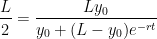
$\displaystyle \frac{L}{2} = A$

This suggests that, as the infection spreads throughout a population, the curve changes concavity at the time that half of the population becomes infected. In other words, the infection spreads fastest throughout the population at the time when half of the population has been infected.

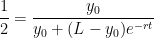
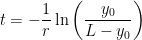
The time at which the point of inflection occurs can be found by setting $A(t) = \displaystyle \frac{L}{2}$ and solving for $t$ :

$\displaystyle \frac{L}{2} = \displaystyle \frac{Ly_0}{y_0+ (L-y_0)e^{-rt}}$ .

$\displaystyle \frac{1}{2} = \displaystyle \frac{y_0}{y_0+ (L-y_0)e^{-rt}}$ .

$y_0 + (L-y_0) e^{-rt} = 2y_0$

$(L-y_0) e^{-rt} = y_0$

$e^{-rt} = \displaystyle \frac{y_0}{L-y_0}$

$-rt = \displaystyle \ln \left( \frac{y_0}{L-y_0} \right)$

$t = \displaystyle - \frac{1}{r} \ln \left( \frac{y_0}{L-y_0} \right)$

This technique for finding the points of inflection directly from the differential equation is possible whenever the differential equation is autonomous, which loosely means that the independent variable does not appear on the right-hand side.

Exponential growth and decay (Part 15): Logistic growth model

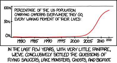
Today, I introduce the logistic growth model, which describes how an infection (like a disease, a rumor, or advertise) spreads in a population. For example:

Sources: http://www.xkcd.com/1220/ and http://www.xkcd.com/1235/

In yesterday’s post, I described an in-class demonstration that engages students while also making the following formula believable:

$A(t) = \displaystyle \frac{L}{1 + (L-1)e^{-rt}}$ .

Where does this formula come from? Suppose that a disease is spreading in a population of size $L$ . It stands to reason that the rate at which the disease spreads is proportional to the number of possible contacts between those who have the disease and those who don’t. If $A(t)$ is the number of people who have the disease, then $L-A(t)$ is the number of people who don’t have the disease. Therefore, the product $A(t) [ L - A(t) ]$ is the number of possible contacts between those who have the disease and those who don’t. This leads to the governing differential equation

$A'(t) = c A(t) [ L - A(t) ]$ ,

where $c$ is the constant of proportionality. This is often rewritten by letting $c = \displaystyle \frac{r}{L}$ , or $r = cL$ :

$A'(t) = \displaystyle \frac{r}{L} A(t) [ L - A(t) ]$

$A'(t) = r A(t) \displaystyle \left[1 - \frac{A(t)}{L} \right]$

The good news is that this differential equation can be solved using separation of variables, just like the governing differential equations for continuous compound interest, paying off credit card debt, radioactive decay, and Newton’s Law of Cooling. The bad news is that it’s a lot harder to calculate the required integrals! After all, the right-hand side, after distributing, has a term containing $A^2$ , which makes this differential equation non-linear.

Solving this differential equation is a bit tedious, and I don’t feel particularly obligated to re-invent the wheel since it can be found several places on the Internet. Suffice it to say that integration by partial fractions and some very tricky algebra is necessary to solve for $A(t)$ and obtain the solution above. Among several different sources (which likely use different letters than the ones I’m using here):

Wikipedia: http://en.wikipedia.org/wiki/Logistic_function#In_ecology:_modeling_population_growth

MathWorld: http://mathworld.wolfram.com/LogisticEquation.html

Exponential growth and decay (Part 14): Logistic growth model

Today, I introduce the logistic growth model, which describes how an infection (like a disease, a rumor, or advertise) spreads in a population. Before I actually present the formula to my students, I usually perform a 8- to 10-minute demonstration to convince students that the formula actually works. This demonstration works well with between 15 and 45 students; I have personally not attempted this demo with a class larger than 45.

I wish I could take credit for the idea behind this demonstration. I’m afraid I can’t remember who told me the idea behind this demo about 15 years ago, but I’m thankful to him or her for this idea, as I’ve used it with great success over the years when teaching Precalculus and even when teaching Differential Equations.

Here’s the demonstration:

1. The class period before the demo, I ask my students to bring their calculators to class.

2. On the day of the demo, I prepare slips of paper with the numbers 1, 2, 3, etc. I hand these to my students as they take their seats before class starts (and, as needed, to students who arrive late).

3. I tell the class that we’re going to model how a rumor gets spread. On the chalkboard, I write down the numbers 0, 1, 2, …, up to $N$ , the number of students in the class that day. Invariably, I get asked, “What’s the rumor?” In response, I’ll playfully point to someone in the front row and say, “The rumor is about him.”

4. I point out that, at time 0, only one person has heard the rumor…. me. I’m person number 0 (confirming the popular belief of my students). So I’ll cross out the 0 on the board and mark on a table that only one person has heard the rumor so far. (Here’s the spreadsheet that I’ve used to keep track of this information while simultaneously making a graph of the data: logisitic).

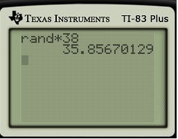
5. I begin to spread the rumor. To spread the rumor, I use my calculator to get a random number between $0$ and $N$ . This can be done by just using the built-in random number generator found on many calculators and then multiplying by $N+1$ . (After all, there are $L= N+1$ people in the room: $N$ students plus one instructor.) The part after the decimal point is not important; the number before the decimal point represents the next person to hear the rumor.

For example, in the figure below, I would tell that person #35 of my class of 37 students was the next to hear the rumor. (If my random number is 0, I’ll privately cheat and get until I get a random number other than 0. I only permit the possibility of cheating on the first step so that the data fits the predicted curve as accurately as possible.)

6. At this point, I’ll X out the number of the next person to hear the rumor (in this case, 35), and I then ask how many people have heard the rumor. Obviously, two people have heard the rumor. So I’ll note on the table that two people have heard the rumor after one step.

7. Now we repeat the process. I get a new random number, and I ask the first student to pull out his/her calculator to get a random number too. But there’s an important rule: if you get a number that’s already been called, that’s OK. This models what really happens when a rumor (or disease) spreads in a population — it’s perfectly possible to hear the rumor twice.

8. We repeat the process — X’ing out numbers that have been previously called and students calling out the next person to hear the rumor — until the entire class hears the rumor. At some point, it becomes easiest to ask students to only call out if they get a number that hasn’t been called yet. Invariably, there’s always one person at the end who hasn’t heard the rumor yet, and this student is often the subject of some good-natured ribbing. Eventually, a chart like the following is produced.

9. Students immediately see that this is a different type of function than pure exponential growth. It actually does start off looking like exponential growth, but at some point the curve levels off. This makes sense because there’s a limiting value of $L=N+1$ (in this case, 38), which can’t happen for a model like $A = A_0 e^{rt}$

10. The punchline is that the spreadsheet secretly computes the actual curve predicted by the logistic growth model. The numbers are actually located in column C, which is conveniently hidden beneath the graph. The function is

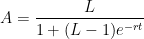
$A = \displaystyle \frac{L}{1 + (L-1)e^{-rt}}$ ,

where $r = \ln 2$ . (Had each person the rumor to two different people at each step, then $r$ would have been equal to $r = \ln 3$ .) Here’s the graph, superimposed upon the data collected from class. I can do this pretty quickly in class because the curve is actually already drawn in the figure above… but it’s drawn in gray, the same color as the background. By changing the color to black, the graph becomes clear:

I never expect the curve to exactly fit the data, but it should come pretty close. After this fairly dramatic revelation, my students are completely sold that the mathematics that I’m about to show them actually works.