Unsolved problems: the Collatz conjecture

Students at all levels — elementary, middle, secondary, and college — tend to think that either (1) all the problems in mathematics have already been solved, or else (2) some unsolved problems remain but only an expert can understand even the statement of the problem.

There are plenty of famous unsolved problems in mathematics. And the Collatz conjecture is an easily stated unsolved problem that can be understood by most fourth and fifth graders.

Here’s the statement of the problem.

Start with any positive integer.
If the integer is even, divide it by $2$ . If it’s odd, multiply it by $3$ and then add $1$ .
Repeat until (and if) you reach $1$ .

That’s it. From Wikipedia:

For instance, starting with 6, one gets the sequence 6, 3, 10, 5, 16, 8, 4, 2, 1.

Starting with 11, for example, takes longer to reach 1: 11, 34, 17, 52, 26, 13, 40, 20, 10, 5, 16, 8, 4, 2, 1.

The sequence for 27 takes 111 steps, climbing to 9232 before descending to 1: 27, 82, 41, 124, 62, 31, 94, 47, 142, 71, 214, 107, 322, 161, 484, 242, 121, 364, 182, 91, 274, 137, 412, 206, 103, 310, 155, 466, 233, 700, 350, 175, 526, 263, 790, 395, 1186, 593, 1780, 890, 445, 1336, 668, 334, 167, 502, 251, 754, 377, 1132, 566, 283, 850, 425, 1276, 638, 319, 958, 479, 1438, 719, 2158, 1079, 3238, 1619, 4858, 2429, 7288, 3644, 1822, 911, 2734, 1367, 4102, 2051, 6154, 3077, 9232, 4616, 2308, 1154, 577, 1732, 866, 433, 1300, 650, 325, 976, 488, 244, 122, 61, 184, 92, 46, 23, 70, 35, 106, 53, 160, 80, 40, 20, 10, 5, 16, 8, 4, 2, 1

The longest progression for any initial starting number less than 100 million is 63,728,127, which has 949 steps. For starting numbers less than 1 billion it is 670,617,279, with 986 steps, and for numbers less than 10 billion it is 9,780,657,630, with 1132 steps.

Here’s the question: Does this sequence eventually reach $1$ no matter the starting value? Or is there a number out there that you could use as a starting value that has a sequence that never reaches $1$ ?

Like I said, this is an easily stated problem that most fourth graders could understand. And no one knows the answer. Every number that’s been tried by computer has produced a sequence that eventually reaches $1$ . But that doesn’t mean that there isn’t a bigger number out there that doesn’t reach $1$ .

I’ll refer to the above Wikipedia page (and references therein) for further reading about the Collatz conjecture. Pedagogically, I suggest that casually mentioning this unsolved problem in class might inspire students to play with mathematics on their own, rather than think that all of mathematics has already been solved by somebody.

Source: http://www.xkcd.com/710/

Reminding students about Taylor series (Part 6)

Sadly, at least at my university, Taylor series is the topic that is least retained by students years after taking Calculus II. They can remember the rules for integration and differentiation, but their command of Taylor series seems to slip through the cracks. In my opinion, the reason for this lack of retention is completely understandable from a student’s perspective: Taylor series is usually the last topic covered in a semester, and so students learn them quickly for the final and quickly forget about them as soon as the final is over.

Of course, when I need to use Taylor series in an advanced course but my students have completely forgotten this prerequisite knowledge, I have to get them up to speed as soon as possible. Here’s the sequence that I use to accomplish this task. Covering this sequence usually takes me about 30 minutes of class time.

I should emphasize that I present this sequence in an inquiry-based format: I ask leading questions of my students so that the answers of my students are driving the lecture. In other words, I don’t ask my students to simply take dictation. It’s a little hard to describe a question-and-answer format in a blog, but I’ll attempt to do this below.

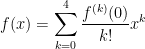
In the previous posts, I described how I lead students to the definition of the Maclaurin series

$f(x) = \displaystyle \sum_{k=0}^{\infty} \frac{f^{(k)}(0)}{k!} x^k$ ,

which converges to $f(x)$ within some radius of convergence for all functions that commonly appear in the secondary mathematics curriculum.

Step 7. Let’s now turn to trigonometric functions, starting with $f(x) = \sin x$ .

What’s $f(0)$ ? Plugging in, we find $f(0) = \sin 0 = 0$ .

As before, we continue until we find a pattern. Next, $f'(x) = \cos x$ , so that $f'(0) = 1$ .

Next, $f''(x) = -\sin x$ , so that $f''(0) = 0$ .

Next, $f'''(x) = -\cos x$ , so that $f''(0) = -1$ .

No pattern yet. Let’s keep going.

Next, $f^{(4)}(x) = \sin x$ , so that $f^{(4)}(0) = 0$ .

Next, $f^{(5)}(x) = \cos x$ , so that $f^{(5)}(0) = 1$ .

Next, $f^{(6)}(x) = -\sin x$ , so that $f^{(6)}(0) = 0$ .

Next, $f^{(7)}(x) = -\cos x$ , so that $f^{(7)}(0) = -1$ .

OK, it looks like we have a pattern… albeit more awkward than the patterns for $e^x$ and $\displaystyle \frac{1}{1-x}$ . Plugging into the series, we find that

$\displaystyle \sin x= x - \frac{x^3}{3!} + \frac{x^5}{5!} - \frac{x^7}{7!} \dots$

If we stare at the pattern of terms long enough, we can write this more succinctly as

$\sin x = \displaystyle \sum_{n=0}^\infty (-1)^n \frac{x^{2n+1}}{(2n+1)!}$

The $(-1)^n$ term accounts for the alternating signs (starting on positive with $n=0$ ), while the $2n+1$ is needed to ensure that each exponent and factorial is odd.

Let’s see… $\sin x$ has a Taylor expansion that only has odd exponents. In what other sense are the words “sine” and “odd” associated?

In Precalculus, a function $f(x)$ is called odd if $f(-x) = -f(x)$ for all numbers $x$ . For example, $f(x) = x^9$ is odd since $f(-x) = (-x)^9 = -x^9$ since 9 is a (you guessed it) an odd number. Also, $\sin(-x) = -\sin x$ , and so $\sin x$ is also an odd function. So we shouldn’t be that surprised to see only odd exponents in the Taylor expansion of $\sin x$ .

A pedagogical note: In my opinion, it’s better (for review purposes) to avoid the $\displaystyle \sum$ notation and simply use the “dot, dot, dot” expression instead. The point of this exercise is to review a topic that’s been long forgotten so that these Taylor series can be used for other purposes. My experience is that the $\displaystyle \sum$ adds a layer of abstraction that students don’t need to overcome for the time being.

Step 8. Let’s now turn try $f(x) = \cos x$ .

What’s $f(0)$ ? Plugging in, we find $f(0) = \cos 1 = 0$ .

Next, $f'(x) = -\sin x$ , so that $f'(0) = 0$ .

Next, $f''(x) = -\cos x$ , so that $f'(0) = -1$ .

It looks like the same pattern of numbers as above, except shifted by one derivative. Let’s keep going.

Next, $f'''(x) = \sin x$ , so that $f'''(0) = 0$ .

Next, $f^{(4)}(x) = \cos x$ , so that $f^{(4)}(0) = 1$ .

Next, $f^{(5)}(x) = -\sin x$ , so that $f^{(5)}(0) = 0$ .

Next, $f^{(6)}(x) = -\cos x$ , so that $f^{(6)}(0) = -1$ .

OK, it looks like we have a pattern somewhat similar to that of $\sin x$, except only involving the even terms. I guess that shouldn’t be surprising since, from precalculus we know that $\cos x$ is an even function since $\cos(-x) = \cos x$ for all $x$ .

Plugging into the series, we find that

$\displaystyle \cos x= 1 - \frac{x^2}{2!} + \frac{x^4}{4!} - \frac{x^6}{6!} \dots$

If we stare at the pattern of terms long enough, we can write this more succinctly as

$\cos x = \displaystyle \sum_{n=0}^\infty (-1)^n \frac{x^{2n}}{(2n)!}$

As we saw with $e^x$ , the above series converge quickest for values of $x$ near $0$ . In the case of $\sin x$ and $\cos x$ , this may be facilitated through the use of trigonometric identities, thus accelerating convergence.

For example, the series for $\cos 1000^o$ will converge quite slowly (after converting $1000^o$ into radians). However, we know that

$\cos 1000^o= \cos(1000^o - 720^o) =\cos 280^o$

using the periodicity of $\cos x$ . Next, since $\latex 280^o$ is in the fourth quadrant, we can use the reference angle to find an equivalent angle in the first quadrant:

$\cos 1000^o = \cos 280^o = \cos(360^o - 80^o) = \cos 80^o$

Finally, using the cofunction identity $\cos x = \sin(90^o - x)$ , we find

$\cos 1000^o = \cos 80^o = sin(90^o - 80^o) = \sin 10^o$ .

In this way, the sine or cosine of any angle can be reduced to the sine or cosine of some angle between $0^o$ and $45^o = \pi/4$ radians. Since $\pi/4 < 1$ , the above power series will converge reasonably rapidly.

Step 10. For the final part of this review, let’s take a second look at the Taylor series

$e^x = \displaystyle 1 + x + \frac{x^2}{2} + \frac{x^3}{3} + \frac{x^4}{4} + \frac{x^5}{5} + \frac{x^6}{6} + \frac{x^7}{7} + \dots$

Just to be silly — for no apparent reason whatsoever, let’s replace $x$ by $ix$ and see what happens:

$e^{ix} = \displaystyle 1 - \frac{x^2}{2!} + \frac{x^4}{4!} - \frac{x^6}{6!} \dots + i \left[\displaystyle x - \frac{x^3}{3!} + \frac{x^5}{5!} - \frac{x^7}{7!} \dots \right]$

after separating the terms that do and don’t have an $i$ .

Hmmmm… looks familiar….

So it makes sense to define

$e^{ix} = \cos x + i \sin x$ ,

which is called Euler’s formula, thus proving an unexpected connected between $e^x$ and the trigonometric functions.

Reminding students about Taylor series (Part 5)

In the previous posts, I described how I lead students to the definition of the Maclaurin series

$f(x) = \displaystyle \sum_{k=0}^{\infty} \frac{f^{(k)}(0)}{k!} x^k$ ,

which converges to $f(x)$ within some radius of convergence for all functions that commonly appear in the secondary mathematics curriculum.

Step 5. That was easy; let’s try another one. Now let’s try $f(x) = \displaystyle \frac{1}{1-x} = (1-x)^{-1}$ .

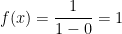
What’s $f(0)$ ? Plugging in, we find $f(x) = \displaystyle \frac{1}{1-0} = 1$ .

Next, to find $f'(0)$ , we first find $f'(x)$ . Using the Chain Rule, we find $f'(x) = -(1-x)^{-2} \cdot (-1) = \displaystyle \frac{1}{(1-x)^2}$ , so that $f'(0) = 1$ .

Next, we differentiate again: $f'(x) = (-2) \cdot (1-x)^{-3} \cdot (-1) = \displaystyle \frac{2}{(1-x)^3}$ , so that $f''(0) = 2$ .

Hmmm… no obvious pattern yet… so let’s keep going.

For the next term, $f'''(x) = (-3) \cdot 2(1-x)^{-4} \cdot (-1) = \displaystyle \frac{6}{(1-x)^4}$ , so that $f'''(0) = 6$ .

For the next term, $f^{(4)}(x) = (-4) \cdot 6(1-x)^{-5} \cdot (-1) = \displaystyle \frac{24}{(1-x)^5}$ , so that $f^{(4)}(0) = 24$ .

Oohh… it’s the factorials again! It looks like $f^{(n)}(0) = n!$ , and this can be formally proved by induction.

Plugging into the series, we find that

$\displaystyle \frac{1}{1-x} = \sum_{n=0}^\infty \frac{n!}{n!} x^n = \sum_{n=0}^\infty x^n = 1 + x + x^2 + x^3 + \dots$ .

Like the series for $e^x$ , this series converges quickest for $x \approx 0$ . Unlike the series for $e^x$ , this series does not converge for all real numbers. As can be checked with the Ratio Test, this series only converges if $|x| < 1$ .

The right-hand side is a special kind of series typically discussed in precalculus. (Students often pause at this point, because most of them have forgotten this too.) It is an infinite geometric series whose first term is $1$ and common ratio $x$. So starting from the right-hand side, one can obtain the left-hand side using the formula

$a + ar + ar^2 + ar^3 + \dots = \displaystyle \frac{a}{1-r}$

by letting $a=1$ and $r=x$. Also, as stated in precalculus, this series only converges if the common ratio satisfies $|r| < 1$, as before.

In other words, in precalculus, we start with the geometric series and end with the function. With Taylor series, we start with the function and end with the series.

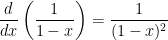
Step 6. A whole bunch of other Taylor series can be quickly obtained from the one for $\displaystyle \frac{1}{1-x}$ . Let’s take the derivative of both sides (and ignore the fact that one should prove that differentiating this infinite series term by term is permissible). Since

$\displaystyle \frac{d}{dx} \left( \frac{1}{1-x} \right) = \frac{1}{(1-x)^2}$

and

$\displaystyle \frac{d}{dx} \left( 1 + x + x^2 + x^3 + x^4 + \dots \right) = 1 + 2x + 3x^2 + 4x^3 + \dots$ ,

we have

$\displaystyle \frac{1}{(1-x)^2} = 1 + 2x + 3x^2 + 4x^3 + \dots$ .

____________________

Next, let’s replace $x$ with $-x$ in the Taylor series in Step 5, obtaining

$\displaystyle \frac{1}{1+x} = 1 - x + x^2 - x^3 + x^4 - x^5 \dots$

Now let’s take the indefinite integral of both sides:

$\displaystyle \int \frac{dx}{1+x} = \int \left( 1 - x + x^2 - x^3 + x^4 - x^5 \dots \right) \, dx$

$\ln(1+x) = \displaystyle x - \frac{x^2}{2} + \frac{x^3}{3} -\frac{ x^4}{4} + \frac{x^5}{5} -\frac{ x^6}{6} \dots + C$

To solve for the constant of integration, let $x = 0$ :

$\ln(1) = 0+ C \Longrightarrow C = 0$

Plugging back in, we conclude that

$\ln(1+x) = x - \displaystyle \frac{x^2}{2} + \frac{x^3}{3} -\frac{ x^4}{4} + \frac{x^5}{5} -\frac{ x^6}{6} \dots$

The Taylor series expansion for $\ln(1-x)$ can be found by replacing $x$ with $-x$ :

$\ln(1-x) = -x - \displaystyle \frac{x^2}{2} - \frac{x^3}{3} -\frac{ x^4}{4} - \frac{x^5}{5} -\frac{ x^6}{6} \dots$

Subtracting, we find

$\ln(1+x) - \ln(1-x) = \ln \displaystyle \left( \frac{1+x}{1-x} \right) = 2x + \frac{2x^3}{3}+ \frac{2x^5}{5} \dots$

My understanding is that this latter series is used by calculators when computing logarithms.

____________________

Next, let’s replace $x$ with $-x^2$ in the Taylor series in Step 5, obtaining

$\displaystyle \frac{1}{1+x^2} = 1 - x^2 + x^4 - x^6 + x^8 - x^{10} \dots$

Now let’s take the indefinite integral of both sides:

$\displaystyle \int \frac{dx}{1+x^2} = \int \left(1 - x^2 + x^4 - x^6 + x^8 - x^{10} \dots\right) \, dx$

$\tan^{-1}x = \displaystyle x - \frac{x^3}{3} + \frac{x^5}{5} -\frac{ x^7}{7} + \frac{x^9}{9} -\frac{ x^{11}}{11} \dots + C$

To solve for the constant of integration, let $x = 0$ :

$\tan^{-1}(1) = 0+ C \Longrightarrow C = 0$

Plugging back in, we conclude that

$\tan^{-1}x = \displaystyle x - \frac{x^3}{3} + \frac{x^5}{5} -\frac{ x^7}{7} + \frac{x^9}{9} -\frac{ x^{11}}{11} \dots$

____________________

In summary, a whole bunch of Taylor series can be extracted quite quickly by differentiating and integrating from a simple infinite geometric series. I’m a firm believer in minimizing the number of formulas that I should memorize. Any time I personally need any of the above series, I’ll quickly use the above steps to derive them from that of $\displaystyle \frac{1}{1-x}$ .

Reminding students about Taylor series (Part 4)

I’m in the middle of a series of posts describing how I remind students about Taylor series. In the previous posts, I described how I lead students to the definition of the Maclaurin series

$f(x) = \displaystyle \sum_{k=0}^{\infty} \frac{f^{(k)}(0)}{k!} x^k$ ,

which converges to $f(x)$ within some radius of convergence for all functions that commonly appear in the secondary mathematics curriculum.

Step 4. Let’s now get some practice with Maclaurin series. Let’s start with $f(x) = e^x$ .

What’s $f(0)$ ? That’s easy: $f(0) = e^0 = 1$ .

Next, to find $f'(0)$ , we first find $f'(x)$ . What is it? Well, that’s also easy: $f'(x) = \frac{d}{dx} (e^x) = e^x$ . So $f'(0)$ is also equal to $1$ .

How about $f''(0)$ ? Yep, it’s also $1$ . In fact, it’s clear that $f^{(n)}(0) = 1$ for all $n$ , though we’ll skip the formal proof by induction.

Plugging into the above formula, we find that

$e^x = \displaystyle \sum_{k=0}^{\infty} \frac{1}{k!} x^k = \sum_{k=0}^{\infty} \frac{x^k}{k!} = 1 + x + \frac{x^2}{2} + \frac{x^3}{3} + \dots$

It turns out that the radius of convergence for this power series is $\infty$ . In other words, the series on the right converges for all values of $x$ . So we’ll skip this for review purposes, this can be formally checked by using the Ratio Test.

At this point, students generally feel confident about the mechanics of finding a Taylor series expansion, and that’s a good thing. However, in my experience, their command of Taylor series is still somewhat artificial. They can go through the motions of taking derivatives and finding the Taylor series, but this complicated symbol in $\displaystyle \sum$ notation still doesn’t have much meaning.

So I shift gears somewhat to discuss the rate of convergence. My hope is to deepen students’ knowledge by getting them to believe that $f(x)$ really can be approximated to high precision with only a few terms. Perhaps not surprisingly, it converges quicker for small values of $x$ than for big values of $x$ .

Pedagogically, I like to use a spreadsheet like Microsoft Excel to demonstrate the rate of convergence. A calculator could be used, but students can see quickly with Excel how quickly (or slowly) the terms get smaller. I usually construct the spreadsheet in class on the fly (the fill down feature is really helpful for doing this quickly), with the end product looking something like this:

In this way, students can immediately see that the Taylor series is accurate to four significant digits by going up to the $x^4$ term and that about ten or eleven terms are needed to get a figure that is as accurate as the precision of the computer will allow. In other words, for all practical purposes, an infinite number of terms are not necessary.

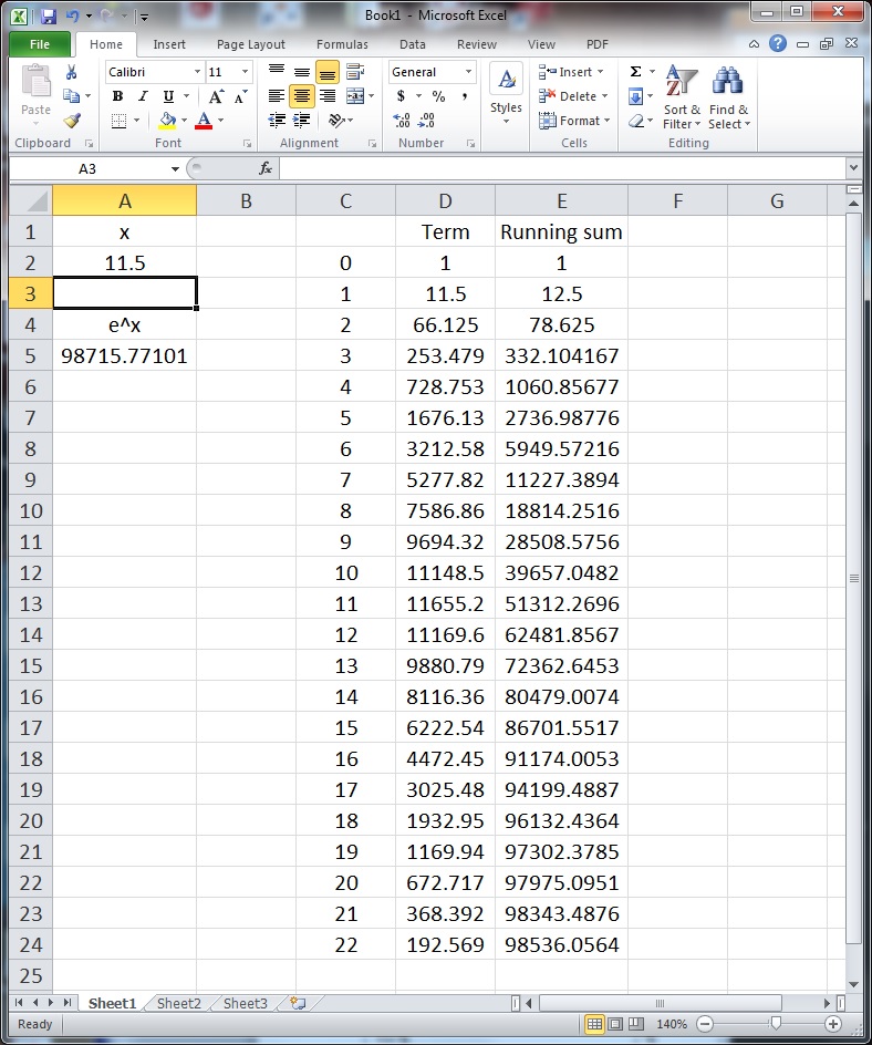
In short, this is how a calculator computes $e^x$ : adding up the first few terms of a Taylor series. Back in high school, when students hit the $e^x$ button on their calculators, they’ve trusted the result but the mechanics of how the calculator gets the result was shrouded in mystery. No longer.

Then I shift gears by trying a larger value of $x$ :

I ask my students the obvious question: What went wrong? They’re usually able to volunteer a few ideas:

The convergence is slower for larger values of $x$ .
The series will converge, but more terms are needed (and I’ll later use the fill down feature to get enough terms so that it does converge as accurate as double precision will allow).
The individual terms get bigger until $k=11$ and then start getting smaller. I’ll ask my students why this happens, and I’ll eventually get an explanation like

$\displaystyle \frac{(11.5)^6}{6!} < \frac{(11.5)^6}{6!} \times \frac{11.5}{7} = \frac{(11.5)^7}{7!}$

but

$\displaystyle \frac{(11.5)^{11}}{11!} < \frac{(11.5)^{11}}{11!} \times \frac{11.5}{12} = \frac{(11.5)^{12}}{12!}$

At this point, I’ll mention that calculators use some tricks to speed up convergence. For example, the calculator can simply store a few values of $e^x$ in memory, like $e^{16}$ , $e^{8}$ , $e^{4}$ , $e^{2}$ , and $e^{1} = e$ . I then ask my class how these could be used to find $e^{11.5}$ . After some thought, they will volunteer that

$e^{11.5} = e^8 \cdot e^2 \cdot e \cdot e^{0.5}$ .

The first three values don’t need to be computed — they’ve already been stored in memory — while the last value can be computed via Taylor series. Also, since $0.5 < 1$ , the series for $e^{0.5}$ will converge pretty quickly. (Some students may volunteer that the above product is logically equivalent to turning $11$ into binary.)

At this point — after doing these explicit numerical examples — I’ll show graphs of $e^x$ and graphs of the Taylor polynomials of $e^x$ , observing that the polynomials get closer and closer to the graph of $e^x$ as more terms are added. (For example, see the graphs on the Wikipedia page for Taylor series, though I prefer to use Mathematica for in-class purposes.) In my opinion, the convergence of the graphs only becomes meaningful to students only after doing some numerical examples, as done above.

At this point, I hope my students are familiar with the definition of Taylor (Maclaurin) series, can apply the definition to $e^x$ , and have some intuition meaning that the nasty Taylor series expression practically means add a bunch of terms together until you’re satisfied with the convergence.

In the next post, we’ll consider another Taylor series which ought to be (but usually isn’t) really familiar to students: an infinite geometric series.

P.S. Here’s the Excel spreadsheet that I used to make the above figures: Taylor.

Reminding students about Taylor series (Part 3)

In the previous post, I described how I lead students to the equations

$f(x) = \displaystyle \sum_{k=0}^n \frac{f^{(k)}(0)}{k!} x^k$ .

and

$f(x) = \displaystyle \sum_{k=0}^n \frac{f^{(k)}(a)}{k!} (x-a)^k$ ,

where $f(x)$ is a polynomial and $a$ can be any number.

Step 3. What happens if the original function $f(x)$ is not a polynomial? For one thing, the right-hand side can no longer be a finite sum. As long as the sum on the right-hand side stops at some degree $n$ , the right-hand side is a polynomial, but the left-hand side is assumed to not be a polynomial.

To resolve this, we can cross our fingers and hope that

$f(x) = \displaystyle \sum_{k=0}^{\infty} \frac{f^{(k)}(0)}{k!} x^k$ ,

$f(x) = \displaystyle \sum_{k=0}^{\infty}\frac{f^{(k)}(a)}{k!} (x-a)^k$ .

In other words, let’s make the right-hand side an infinite series, and hope for the best. This is the definition of the Taylor series expansions of $f$ .

Note: At this point in the review, I can usually see the light go on in my students’ eyes. Usually, they can now recall their work with Taylor series in the past… and they wonder why they weren’t taught this topic inductively (like I’ve tried to do in the above exposition) instead of deductively (like the presentation in most textbooks).

While we’d like to think that the Taylor series expansions always work, there are at least two things that can go wrong.

First, the sum on the left is an infinite series, and there’s no guarantee that the series will converge in the first place. There are plenty of example of series that diverge, like $\displaystyle \sum_{k=0}^\infty \frac{1}{k+1}$ .
Second, even if the series converges, there’s no guarantee that the series will converge to the “right” answer $f(x)$ . The canonical example of this behavior is $f(x) = e^{-1/x^2}$ , which is so “flat” near $x=0$ that every single derivative of $f$ is equal to $0$ at $x =0$ .

For the first complication, there are multiple tests devised in Calculus II, especially the Ratio Test, to determine the values of $x$ for which the series converges. This establishes a radius of convergence for the series.

The second complication is far more difficult to address rigorously. The good news is that, for all commonly occurring functions in the secondary mathematics curriculum, the Taylor series of a function properly converges (when it does converge). So we will happily ignore this complication for the remainder of the presentation.

Indeed, it’s remarkable that the series should converge to $f(x)$ at all. Think about the meaning of the terms on the right-hand side:

$f(a)$ is the $y-$ coordinate at $x=a$ .
$f'(a)$ is the slope of the curve at $x=a$ .
$f''(a)$ is a measure of the concavity of the curve at — you guessed it — $x=a$ .
$f'''(a)$ is an even more subtle description of the curve… once again, at $x=a$ .

In other words, if the Taylor series converges to $f(x)$ , then every twist and turn of the function, even at points far away from $x=a$ , is encoded somehow in the shape of the curve at the one point $x=a$ . So analytic functions (which has a Taylor series which converges to the original functions) are indeed quite remarkable.

Reminding students about Taylor series (Part 2)

In this series of posts, I will describe the sequence of examples that I use to remind students about Taylor series. (One time, just for fun, I presented this topic at the end of a semester of Calculus I, and it seemed to go well even for that audience who had not seen Taylor series previously.)

I should emphasize that I present this sequence inductively and in an inquiry-based format: I ask leading questions of my students so that the answers of my students are driving the lecture. In other words, I don’t ask my students to simply take dictation. It’s a little hard to describe a question-and-answer format in a blog, but I’ll attempt to do this below.

Step 1. Find the unique quartic (fourth-degree) polynomial so that $f(0) = 6$ , $f'(0) = -3$ , $f''(0) = 6$ , $f'''(0) = 2$ , and $f^{(4)}(0) = 10$ .

I’ve placed a thought bubble if you’d like to think about it before scrolling down to see the answer. Here’s a hint to get started: let $f(x) = ax^4 + bx^3 + cx^2 + dx + e$ , and start differentiating. Remember that $a$ , $b$ , $c$ , $d$ , and $e$ are constants.

We begin with the information that $f(0) = 6$ . How else can we find $f(0)$? Since $f(x) = ax^4 + bx^3 + cx^2 + dx + e$ , we see that $f(0) = e$ . Therefore, it must be that $e = 6$ .

How about $f'(0)$ ? We see that $f'(x) = 4ax^3 + 3bx^2 + 2cx + d$ , and so $f'(0) = d$ . Since $f'(0) = -3$ , we have that $d = -3$ .

Next, $f''(x) = 12ax^2 + 6bx + 2c$ , and so $f''(0) = 2c$ . Since $f''(0) = 6$ ,we have that $2c = 6$ , or $c = 3$ .

Next, $f'''(x) = 24ax + 6b$ , and so $f'''(0) = 6b$ . Since $f'''(0) = 2$ ,we have that $6b = 2$ , or $b = \frac{1}{3}$ .

Finally, $f^{(4)}(x) = 24a$ , and so $f^{(4)}(0) = 24a$ . Since $f^{(4)}(0) = 10$ , we have $24a = 10$ , or $a = \frac{5}{12}$ .

What do we get when we put all of this information together? The polynomial must be

$f(x) = \frac{5}{12} x^4 + \frac{1}{3} x^3 + 3 x^2 - 3x + 6$ .

Step 2. How are these coefficients related to the information given in the problem?

Let’s start with the leading coefficient, $a = \frac{5}{12}$ . How did we get this answer? It came from dividing $10$ by $24$ . Where did the $10$ come from? It was the given value of $f^{(4)}(0)$ , and so

$a = \displaystyle \frac{f^{(4)}(0)}{24}$ .

Next, $b = \frac{1}{3}$ , which arose from dividing $2$ by $6$ . The number $2$ was the given value of $f'''(0)$ , and so

$b =\displaystyle \frac{f'''(0)}{6}$ .

Moving to the next coefficient, $c = 3$ , which arose from dividing $f''(0) = 6$ by $2$ . So

$c = \displaystyle\frac{f''(0)}{2}$ .

Finally, it’s clear that

$d = f'(0)$ and $e = f(0)$ .

This last line doesn’t quite fit the pattern of the first three lines. The first three lines all have fractions, but these last two expressions don’t. How can we fix this? In the hopes of finding a pattern, let’s (unnecessarily) write $d$ and $e$ as fractions by dividing by $1$ :

$d = \displaystyle\frac{f'(0)}{1}$ and $e = \displaystyle \frac{f(0)}{1}$ .

Let’s now rewrite the polynomial $f(x)$ in light of this discussion:

$f(x) = \displaystyle \frac{f'^{(4)}(0)}{24} x^4 + \frac{f'''(0)}{6} x^3 + \frac{f'''(0)}{2} x^2 + \frac{f'(0)}{1}x + \frac{f(0)}{1}$ .

What pattern do we see in the numerators? It’s apparent that the number of derivatives matches the power of $x$ . For example, the $x^3$ term has a coefficient involving the third derivative of $f$ . The last two terms fit this pattern as well, since $x = x^1$ and the last term is multiplied by $x^0 = 1$ .

What pattern do we see in the denominators? $1, 1, 2, 6, 24 \dots$ where have we seen those before? Oh yes, the factorials! We know that $4! = 4 \cdot 3 \cdot 2 \cdot 1 = 24$ , $3! = 3 \cdot 2 \cdot 1 = 6$ , $2! = 2 \cdot 1 = 2$ , $1! = 1$ , and $0!$ is defined to be $1$ . So $f(x)$ can be rewritten as

$f(x) = \displaystyle \frac{f'^{(4)}(0)}{4!} x^4 + \frac{f'''(0)}{3!} x^3 + \frac{f'''(0)}{2!} x^2 + \frac{f'(0)}{1!}x + \frac{f(0)}{0!}$ .

How can this be written more compactly? By using $\displaystyle \sum-$ notation:

$f(x) = \displaystyle \sum_{k=0}^4 \frac{f^{(k)}(0)}{k!} x^k$ .

Why does the sum stop at 4? Because the original polynomial had degree 4. In general, if the polynomial had degree $n$ , it’s reasonable to guess that

$f(x) = \displaystyle \sum_{k=0}^n \frac{f^{(k)}(0)}{k!} x^k$ .

This is called the Maclaurian series, or the Taylor series about $x =0$ . While I won’t prove it here, one can find Taylor series expansions about points other than $0$ :

$f(x) = \displaystyle \sum_{k=0}^n \frac{f^{(k)}(a)}{k!} (x-a)^k$ ,

where $a$ can be any number. Though not proven here, these series are exactly true for polynomials.

In the next post, we’ll discuss what happens if $f(x)$ is not a polynomial.

Reminding students about Taylor series (Part 1)

At my university, Calculus II covers approximately the same topics covered in an AP Calculus BC course: integrals and derivatives with logarithms and exponential functions, various techniques of integration (including integration by parts and trigonometric substitutions), and convergence of infinite series.

In my opinion, the single most important of these topics is Taylor series (or, if you prefer, Maclaurin series), as these approximations to transcendental functions like $e^x$ and $\sin x$ are used over and over again in higher mathematics.

$\bullet$ A good working knowledge of Taylor series is necessary for computing series solutions of ordinary differential equations.

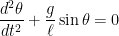
$\bullet$ In physics, elementary approximations like $\sin x \approx x$ are used over and over again. For example, the governing differential equation for the motion of oscillating pendulums is

$\displaystyle \frac{d^2 \theta}{dt^2} + \frac{g}{\ell} \sin \theta = 0$ ,

where $g$ is the acceleration due to gravity and $\ell$ is the length of the pendulum. This differential equation cannot be solved exactly, and its solution is very complex.

However, for small angles, we may use the approximation $\sin \theta \approx \theta$ , so that the differential equation becomes

$\displaystyle \frac{d^2 \theta}{dt^2} + \frac{g}{\ell} \theta = 0$ ,

By eliminating the $\sin \theta$ term, we now have a second-order differential equation with constant coefficients, which can be solved in a straightforward manner using standard techniques from differential equations. If $\theta(0) = \theta_0$ and $\theta'(0) = 0$ (i.e., the pendulum is pulled a small angle $\theta_0$ and is then released), the solution is

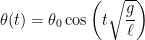
$\theta(t) = \theta_0 \cos\left(t \sqrt{\displaystyle \frac{g}{\ell}} \right)$ .

In other words, the pendulum exhibits sinusoidal behavior. (FYI, for an amazing display of kinetic art, see this demonstration of pendulum waves.)

$\bullet$ The primary way that students interface with Taylor series is through their calculators. When a calculator computes $\cos 1000^o$ , it doesn’t draw a unit circle, trace out an angle of $1000^o$ in standard position, and find the $x-$ coordinate of the terminal point. Instead, the calculator converts $1000^o$ into radians and adds the first few terms of the Taylor series expansion for $\cos x.$

The calculator may use a few tricks to accelerate convergence. For this example, using some trigonometric identities, $\cos 1000^o= \cos 280^o= \cos 80^o= \sin 10^o$ , and (as I’ll discuss) the Maclaurin series for $\sin x$ at $x = 10^o$ converges much faster than the Maclaurin series for $\cos x$ at $x = 1000^o$ .

I’ve argued the importance of Taylor series in higher-level courses in both mathematics and physics. Sadly, at least at my university, Taylor series is probably the topic that is least retained by students years after taking Calculus II. They can remember the rules for integration and differentiation, but their command of Taylor series seems to slip through the cracks.

In my opinion, the reason for this lack of retention is completely understandable from a student’s perspective: Taylor series is usually the last topic covered in a semester, and so students learn them quickly for the final and quickly forget about them as soon as the final is over.

Of course, when I need to use Taylor series in an advanced course but my students have completely forgotten this prerequisite knowledge, I have to get them up to speed as soon as possible. Over the next few posts, I will present the sequence of examples that I use to accomplish this task. Covering this sequence usually takes me about 30-40 minutes of class time, depending on the class.

I should emphasize that, as much as possible, I present this sequence inductively and in an inquiry-based format: I ask leading questions of my students so that the answers of my students are driving the lecture. In other words, I don’t ask my students to simply take dictation. It’s a little hard to describe a question-and-answer format in a blog, but I’ll attempt to do this below.

Beginning with the next post, I’ll describe this sequence.

Welch’s formula

When conducting an hypothesis test or computing a confidence interval for the difference $\overline{X}_1 - \overline{X}_2$ of two means, where at least one mean does not arise from a small sample, the Student t distribution must be employed. In particular, the number of degrees of freedom for the Student t distribution must be computed. Many textbooks suggest using Welch’s formula:

$df = \frac{\displaystyle (SE_1^2 + SE_2^2)^2}{\displaystyle \frac{SE_1^4}{n_1-1} + \frac{SE_2^4}{n_2-1}},$

rounded down to the nearest integer. In this formula, $SE_1 = \displaystyle \frac{\sigma_1}{\sqrt{n_1}}$ is the standard error associated with the first average $\overline{X}_1$ , where $\sigma_1$ (if known) is the population standard deviation for $X$ and $n_1$ is the number of samples that are averaged to find $\overline{X}_1$ . In practice, $\sigma_1$ is not known, and so the bootstrap estimate $\sigma_1 \approx s_1$ is employed.

The terms $SE_2$ and $n_2$ are similarly defined for the average $\overline{X}_2$ .

In Welch’s formula, the term $SE_1^2 + SE_2^2$ in the numerator is equal to $\displaystyle \frac{\sigma_1^2}{n_1} + \frac{\sigma_2^2}{n_2}$ . This is the square of the standard error $SE_D$ associated with the difference $\overline{X}_1 - \overline{X}_2$ , since

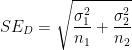
$SE_D = \displaystyle \sqrt{\frac{\sigma_1^2}{n_1} + \frac{\sigma_2^2}{n_2}}$ .

This leads to the “Pythagorean” relationship

$SE_1^2 + SE_2^2 = SE_D^2$ ,

which (in my experience) is a reasonable aid to help students remember the formula for $SE_D$ .

Naturally, a big problem that students encounter when using Welch’s formula is that the formula is really, really complicated, and it’s easy to make a mistake when entering information into their calculators. (Indeed, it might be that the pre-programmed calculator function simply gives the wrong answer.) Also, since the formula is complicated, students don’t have a lot of psychological reassurance that, when they come out the other end, their answer is actually correct. So, when teaching this topic, I tell my students the following rule of thumb so that they can at least check if their final answer is plausible:

$\min(n_1,n_2)-1 \le df \le n_1 + n_2 -2$ .

To my surprise, I have never seen this formula in a statistics textbook, even though it’s quite simple to state and not too difficult to prove using techniques from first-semester calculus.

Let’s rewrite Welch’s formula as

$df = \left( \displaystyle \frac{1}{n_1-1} \left[ \frac{SE_1^2}{SE_1^2 + SE_2^2}\right]^2 + \frac{1}{n_2-1} \left[ \frac{SE_2^2}{SE_1^2 + SE_2^2} \right]^2 \right)^{-1}$

For the sake of simplicity, let $m_1 = n_1 - 1$ and $m_2 = n_2 -1$ , so that

$df = \left( \displaystyle \frac{1}{m_1} \left[ \frac{SE_1^2}{SE_1^2 + SE_2^2}\right]^2 + \frac{1}{m_2} \left[ \frac{SE_2^2}{SE_1^2 + SE_2^2} \right]^2 \right)^{-1}$

Now let $x = \displaystyle \frac{SE_1^2}{SE_1^2 + SE_2^2}$ . All of these terms are nonnegative (and, in practice, they’re all positive), so that $x \ge 0$ . Also, the numerator is no larger than the denominator, so that $x \le 1$ . Finally, we notice that

$1-x = 1 - \displaystyle \frac{SE_1^2}{SE_1^2 + SE_2^2} = \frac{SE_2^2}{SE_1^2 + SE_2^2}$ .

Using these observations, Welch’s formula reduces to the function

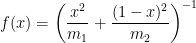
$f(x) = \left( \displaystyle \frac{x^2}{m_1} + \frac{(1-x)^2}{m_2} \right)^{-1}$ ,

and the central problem is to find the maximum and minimum values of $f(x)$ on the interval $0 \le x \le 1$ . Since $f(x)$ is differentiable on $[0,1]$ , the absolute extrema can be found by checking the endpoints and the critical point(s).

First, the endpoints. If $x=0$ , then $f(0) = \left( \displaystyle \frac{1}{m_2} \right)^{-1} = m_2$ . On the other hand, if $x=1$ , then $f(1) = \left( \displaystyle \frac{1}{m_1} \right)^{-1} = m_1$ .

Next, the critical point(s). These are found by solving the equation $f'(x) = 0$ :

$f'(x) = -\left( \displaystyle \frac{x^2}{m_1} + \frac{(1-x)^2}{m_2} \right)^{-2} \left[ \displaystyle \frac{2x}{m_1} - \frac{2(1-x)}{m_2} \right] = 0$

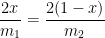
$\displaystyle \frac{2x}{m_1} - \frac{2(1-x)}{m_2} = 0$

$\displaystyle \frac{2x}{m_1} = \frac{2(1-x)}{m_2}$

$xm_2= (1-x)m_1$

$xm_2 = m_1 - xm_1$

$x(m_1 + m_2) = m_1$

$x = \displaystyle \frac{m_1}{m_1 + m_2}$

Plugging back into the original equation, we find the local extremum

$f \left( \displaystyle \frac{m_1}{m_1+m_2} \right) = \left( \displaystyle \frac{1}{m_1} \frac{m_1^2}{(m_1+m_2)^2} + \frac{1}{m_2} \left[1-\frac{m_1}{m_1+m_2}\right]^2 \right)^{-1}$

$f \left( \displaystyle \frac{m_1}{m_1+m_2} \right) = \left( \displaystyle \frac{1}{m_1} \frac{m_1^2}{(m_1+m_2)^2} + \frac{1}{m_2} \left[\frac{m_2}{m_1+m_2}\right]^2 \right)^{-1}$

$f \left( \displaystyle \frac{m_1}{m_1+m_2} \right) = \left( \displaystyle \frac{m_1}{(m_1+m_2)^2} + \frac{m_2}{(m_1+m_2)^2} \right)^{-1}$

$f \left( \displaystyle \frac{m_1}{m_1+m_2} \right) = \left( \displaystyle \frac{m_1+m_2}{(m_1+m_2)^2} \right)^{-1}$

$f \left( \displaystyle \frac{m_1}{m_1+m_2} \right) = \left( \displaystyle \frac{1}{m_1+m_2} \right)^{-1}$

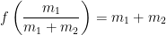
$f \left( \displaystyle \frac{m_1}{m_1+m_2} \right) = m_1+m_2$

Based on the three local extrema that we’ve found, it’s clear that the absolute minimum of $f(x)$ on $[0,1]$ is the smaller of $m_1$ and $m_2$ , while the absolute maximum is equal to $m_1 + m_2$ .

$\hbox{QED}$

In conclusion, I suggest offering the following guidelines to students to encourage their intuition about the plausibility of their answers:

If $SE_1$ is much smaller than $SE_2$ (i.e., $x \approx 0$ ), then $df$ will be close to $m_2 = n_2 - 1$ .
If $SE_1$ is much larger than $SE_2$ (i.e., $x \approx 1$ ), then $df$ will be close to $m_1 = n_1 - 1$ .
Otherwise, $df$ could be as large as $m_1 + m_2 = n_1 + n_2 - 2$ , but no larger.

More on divisibility

Based on my students’ reactions, I gave my best math joke in years as I went over the proofs for checking that an integer was a multiple of 3 or a multiple of 9. I started by proving a lemma that 9 is always a factor of $10^k - 1$ . I asked my students how I’d write out $10^k - 1$ , and they correctly answered $99{\dots}9$ , a numeral with $k$ consecutive $9$ s. So I said, “Who let the dogs out? Me. See: $k$ nines.”

Some of my students laughed so hard that they cried.

There are actually at least three ways of proving this lemma. I love lemmas like these, as they offer a way of, in the words of my former professor Arnold Ross, to think deeply about simple things.

(1) By subtracting, $10^k - 1 = 99{\dots}9 = 9 \times 11{\dots}1$ , which is clearly a multiple of 9.

(2) We can use the rule

$a^k - b^k = (a-b) \left(a^{k-1} + a^{k-2} b + \dots + a b^{k-2} + b^{k-1} \right)$

The conclusion follows by letting $a = 10$ and $b =1$ .

From my experience, my senior math majors all learned the rule for factoring the difference of two squares, but very few learned the rule for factoring the difference of two cubes, while almost none of them learned the general factorization rule above. As always, it’s not my students’ fault that they weren’t taught these things when they were younger.

I also supplement this proof with a challenge to connect Proof #2 with Proof #1… why does $11{\dots}1 = \left(a^{k-1} + a^{k-2} b + \dots + a b^{k-2} + b^{k-1} \right)$ ?

(3) We can use mathematical induction.

If $k = 0$ , then $10^k - 1 = 0$ , which is a multiple of 9.

We now assume that $10^k - 1$ is a multiple of 9.

To show that $10^{k+1}-1$ is a multiple of 9, we observe that

$10^{k+1}-1 = \left(10^{k+1} - 10^k \right) + \left(10^k - 1\right) = 10^k (10-1) + \left(10^k - 1\right)$ ,

and both terms on the right-hand side are multiples of 9. (I also challenge my students to connect the right-hand side with the original expression $99{\dots}9$ .)

$\hbox{QED}$

A mathematical magic trick

In case anyone’s wondering, here’s a magic trick that I did my class for future secondary math teachers while dressed as Carnac the Magnificent. I asked my students to pull out a piece of paper, a pen or pencil, and (if they wished) a calculator. Here were the instructions I gave them:

Write down just about any number you want. Just make sure that the same digit repeated (not something like 88,888). You may want to choose something that can be typed into a calculator.
Scramble the digits of your number, and write down the new number. Just be sure that any repeated digits appear the same number of times. (For example, if your first number was 1,232, your second number could be 2,231 or 1,322.)
Subtract the smaller of the two numbers from the bigger, and write down the difference. Use a calculator if you wish.
Pick any nonzero digit in the difference, and scratch it out.
Add up the remaining digits (that weren’t scratched out).

I asked my students one at a time what they got after Step 5, and I responded, as the magician, with the number that they had scratched out. One student said 34, and I answered 2. Another said 24, and I answered 3. After doing this a couple more times, one student simply stated, “My mind is blown.”

This is actually a simple trick to perform, and the mathematics behind the trick is fairly straightforward to understand. Based on personal experience, this is a great trick to show children as young as 2nd or 3rd grade who have figured out multiple-digit subtraction and single-digit multiplication.

I offer the following thought bubble if you’d like to think about it before looking ahead to find the secret to this magic trick.

What the magician does: the magician finds the next multiple of 9 greater than the volunteer’s number, and answers with the difference. For example, if the volunteer answers 25, the magician figures out that the next multiple of 9 after 25 is 27. So 27-25 = 2 was the digit that was scratched out.

This trick works because of two important mathematical facts.

(1) The difference $D$ between the original number and the scrambled number is always a multiple of 9. For example, suppose the volunteer chooses 3417, and suppose the scrambled number is 7431. Then the difference is

$7431 - 3417 = (7000 + 400 + 30 + 1) - (3000 + 400 + 10 + 7)$

$= (7000 - 7) + (400 - 400) + (30 - 3000) + (1 - 10)$

$= 7 \times (1000-1) + 4 \times (100-100) + 3 \times (10-1000) + 1 \times (1-10)$

$= 7 \times (999) + 1 \times (0) + 4 \times (-990) + 3 \times (-9)$

Each of the numbers in parentheses is a multiple of 9, and so the difference $D$ must also be a multiple of 9.

A more algebraic proof of (1) is set apart in the block quote below; feel free to skip it if the above numerical example is convincing enough.

More formally, suppose that the original number is $a_n a_{n-1} \dots a_1a_0$ in base-10 notation, and suppose the scrambled number is $a_{\sigma(n)} a_{\sigma(n-1)} \dots a_{\sigma(1)} a_{\sigma(0)}$ , where $\sigma$ is a permutation of the numbers $\{0, 1, \dots, n\}$ . Without loss of generality, suppose that the original number is larger. Then the difference $D$ is equal to

$D = a_n a_{n-1} \dots a_1a_0 - a_{\sigma(n)} a_{\sigma(n-1)} \dots a_{\sigma(1)} a_{\sigma(0)}$

$D = \displaystyle \sum_{i=0}^n a_i 10^i - \sum_{i=0}^n a_{\sigma(i)} 10^i$

$D = \displaystyle \sum_{i=0}^n a_{\sigma(i)} 10^{\sigma(i)} - \sum_{i=0}^n a_{\sigma(i)} 10^i$

$D = \displaystyle \sum_{i=0}^n a_{\sigma(i)} \left(10^{\sigma(i)} - 10^i \right)$

The transition from the second to the third line work because the terms of the first sum are merely rearranged by the permutation $\sigma$ .

To show that $D$ is a multiple of 9, it suffices to show that each term $10^{\sigma(i)} - 10^i$ is a multiple of 9.

If $\sigma(i) > i$ , then $10^{\sigma(i)} - 10^i = 10^i \left( 10^{\sigma(i) - i} - 1 \right)$ , and the term in parentheses is guaranteed to be a multiple of 9.

If $\sigma(i) < i$ , then $10^{\sigma(i)} - 10^i = 10^{\sigma(i)} \left( 1-10^{i-\sigma(i)} \right) = -10^{\sigma(i)} \left( 10^{i-\sigma(i)} - 1 \right)$ , and the term in parentheses is guaranteed to be a (negative) multiple of 9.

If $\sigma(i) = i$ , then $10^{\sigma(i)} - 10^i = 0$ , a multiple of 9.

$\hbox{QED}$

Because the difference $D$ is a multiple of 9, we use the important fact (2) that a number is a multiple of 9 exactly when the sum of its digits is a multiple of 9. Therefore, when the volunteer offers the sum of all but one of the digits of $D$ , the missing digit is found by determining the nonzero number that has to be added to get the next multiple of 9. (Notice that the trick specifies that the volunteer scratch out a nonzero digit. Otherwise, there would be an ambiguity if the volunteer answered with a multiple of 9; the missing digit could be either 0 or 9.)

As I mentioned earlier, I showed this trick (and the proof of why it works) to a class of senior math majors who are about to become secondary math teachers. I think it’s a terrific and engaging way of deepening their content knowledge (in this case, base-10 arithmetic and the rule of checking that a number is a multiple of 9.)

As thanks for reading this far, here’s a photo of me dressed as Carnac as I performed the magic trick. Sadly, most of the senior math majors of 2013 were in diapers when Johnny Carson signed off the Tonight Show in 1992, so they didn’t immediately get the cultural reference.