

Category: Theorems
Inverse Functions: Logarithms and Complex Numbers (Part 30)
Ordinarily, there are no great difficulties with logarithms as we’ve seen with the inverse trigonometric functions. That’s because the graph of 



and we don’t have to worry about “other” solutions.
However, this goes out the window if we consider logarithms with complex numbers. Recall that the trigonometric form of a complex number 

where 


Over the past few posts, we developed the following theorem for computing 

Definition. Let 


Of course, this looks like what the definition ought to be if one formally applies the Laws of Logarithms to 

This is analogous to another situation when an inverse function is defined using a restricted domain, like

or

The Laws of Logarithms also may not work when nonpositive numbers are used. For example,
![\log \left[ (-1) \cdot (-1) \right] = \log 1 = 0](https://s0.wp.com/latex.php?latex=%5Clog+%5Cleft%5B+%28-1%29+%5Ccdot+%28-1%29+%5Cright%5D+%3D+%5Clog+1+%3D+0&bg=ffffff&fg=000000&s=0&c=20201002)
but


This material appeared in my previous series concerning calculators and complex numbers: https://meangreenmath.com/2014/07/09/calculators-and-complex-numbers-part-21/
Proof without words: Pythagoras for a clipped rectangle

2014 MacArthur “Genius” grant winner and the twin prime conjecture
From http://www.macfound.org/fellows/927/:
Prime numbers have inspired great intrigue over the last centuries, and one of the most basic unanswered questions has been the spacing between two consecutive prime numbers, or the twin prime conjecture, which states that there are infinitely many pairs of primes that differ by two. Despite many efforts at proving this conjecture, mathematicians were not able to rule out the possibility that the gaps between primes continue to expand, eventually exceeding any particular bound. Zhang’s work shows that there are infinitely many consecutive primes, or pairs of primes, closer than 70 million. In other words, as you go to larger and larger numbers, the primes will not become further and further apart—you will keep finding prime pairs that differ by less than 70 million.
His work has generated significant collaborations across the community to expand on his effort, and within months of his discovery that number was reduced from 70 million to less than 5,000.
Introduction to knot theory
The Mathematical Association of America has an excellent series of 10-minute lectures on various topics in mathematics that are nevertheless accessible to the general public, including gifted elementary school students. The video below is a gentle introduction to knot theory, including computational issues and 3D printing. From the YouTube description:
Laura Taalman, a professor in the Department of Mathematics and Statistics at James Madison University, discusses using technology to explore mathematics.
Different definitions of e (Part 12): Numerical computation
In this series of posts, we have seen that the number 
1. 
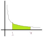 2. We have the limits

These limits form the logical basis for the continuous compound interest formula.
3. We have also shown that 


Therefore, we can let 


In yesterday’s post, I showed that using the original definition (in terms of an area under a hyperbola) does not lend itself well to numerically approximating
2. The limit 
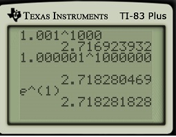 3. The best way to compute



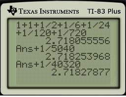
More about approximating
Different definitions of e (Part 11): Numerical computation
In this series of posts, we have seen that the number
1. 2. We have the limits
These limits form the logical basis for the continuous compound interest formula.
3. We have also shown that
Therefore, we can let
Let’s now consider how the decimal expansion of
1. Finding ![[1,1.8]](https://s0.wp.com/latex.php?latex=%5B1%2C1.8%5D&bg=ffffff&fg=000000&s=0&c=20201002)
![[1.8,2.6]](https://s0.wp.com/latex.php?latex=%5B1.8%2C2.6%5D&bg=ffffff&fg=000000&s=0&c=20201002)
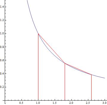
Each trapezoid has a (horizontal) height of 




However, the number 

In other words, we know that the area between 
Great, so 


By either guessing and checking — or with the help of Mathematica — it can be determined that this function of 

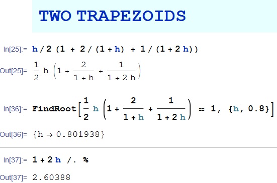
We can try to better with additional trapezoids. With four trapezoids, we can establish that 
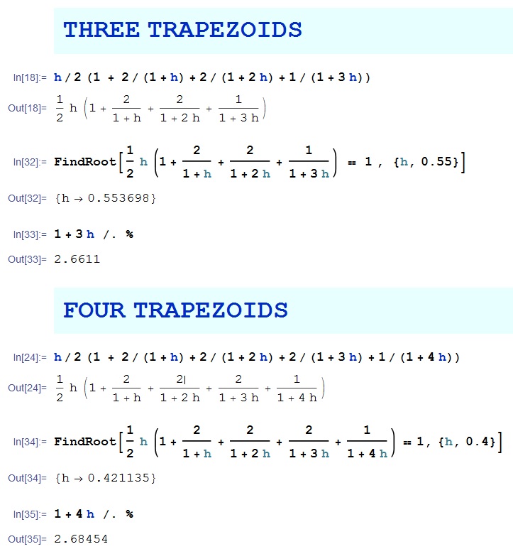
With 100 trapezoids, we can show that 
 However, trapezoids can only provide a lower bound on
To obtain an upper bound on 


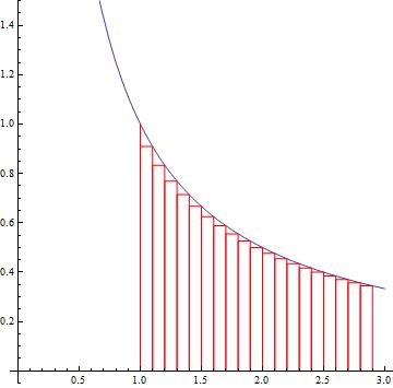 The rectangles all lie below the hyperbola. The width of each one is



In other words, we know that the area between 

Once again, additional rectangles can provide better and better upper bounds on

It then becomes necessary to plug in numbers for
 So with 100 rectangles, we can establish that

Clearly, this is a lot of work for approximating 


In the next post, we’ll explore the other two ways of thinking about the number
Different definitions of e (Part 10): Connecting the two definitions
In this series of posts, I consider how two different definitions of the number
- Algebra II/Precalculus: If
dollars are invested at interest rate
for
years with continuous compound interest, then the amount of money after
.
- Calculus: The number
is equal to

These two definitions appear to be very, very different. One deals with making money. The other deals with the area under a hyperbola. Amazingly, these two definitions are related to each other. In this series of posts, I’ll discuss the connection between the two.
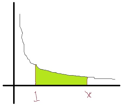
In yesterday’s post, I proved the following theorem, thus completing a long train of argument that began with the second definition of
Theorem. 
Proof #2. Let’s write the left-hand side as

Let’s take the natural logarithm of both sides:
![\ln L = \displaystyle \ln \left[ \lim_{n \to \infty} P \left( 1 + \frac{r}{n} \right)^{nt} \right]](https://s0.wp.com/latex.php?latex=%5Cln+L+%3D+%5Cdisplaystyle+%5Cln+%5Cleft%5B+%5Clim_%7Bn+%5Cto+%5Cinfty%7D+P+%5Cleft%28+1+%2B+%5Cfrac%7Br%7D%7Bn%7D+%5Cright%29%5E%7Bnt%7D+%5Cright%5D&bg=ffffff&fg=000000&s=0&c=20201002)
Since 
![\ln L = \displaystyle \lim_{n \to \infty} \ln \left[ P \left( 1 + \frac{r}{n} \right)^{nt} \right]](https://s0.wp.com/latex.php?latex=%5Cln+L+%3D+%5Cdisplaystyle+%5Clim_%7Bn+%5Cto+%5Cinfty%7D+%5Cln+%5Cleft%5B+P+%5Cleft%28+1+%2B+%5Cfrac%7Br%7D%7Bn%7D+%5Cright%29%5E%7Bnt%7D+%5Cright%5D&bg=ffffff&fg=000000&s=0&c=20201002)
![\ln L = \displaystyle \lim_{n \to \infty} \left[ \ln P + \ln \left( 1 + \frac{r}{n} \right)^{nt} \right]](https://s0.wp.com/latex.php?latex=%5Cln+L+%3D+%5Cdisplaystyle+%5Clim_%7Bn+%5Cto+%5Cinfty%7D+%5Cleft%5B+%5Cln+P+%2B+%5Cln+%5Cleft%28+1+%2B+%5Cfrac%7Br%7D%7Bn%7D+%5Cright%29%5E%7Bnt%7D+%5Cright%5D&bg=ffffff&fg=000000&s=0&c=20201002)
![\ln L = \displaystyle \lim_{n \to \infty} \left[ \ln P + nt \ln \left( 1 + \frac{r}{n} \right)\right]](https://s0.wp.com/latex.php?latex=%5Cln+L+%3D+%5Cdisplaystyle+%5Clim_%7Bn+%5Cto+%5Cinfty%7D+%5Cleft%5B+%5Cln+P+%2B+nt+%5Cln+%5Cleft%28+1+%2B+%5Cfrac%7Br%7D%7Bn%7D+%5Cright%29%5Cright%5D&bg=ffffff&fg=000000&s=0&c=20201002)


The limit on the right-hand side follows the indeterminate form 

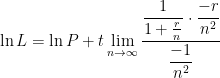

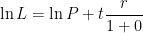

We now solve for the original limit 


Different definitions of e (Part 9): Connecting the two definitions
In this series of posts, I consider how two different definitions of the number
- Algebra II/Precalculus: If
- Calculus: The number
These two definitions appear to be very, very different. One deals with making money. The other deals with the area under a hyperbola. Amazingly, these two definitions are related to each other. In this series of posts, I’ll discuss the connection between the two.
We begin with the second definition, which is usually considered the true definition of


beginning with this definition of the number
Theorem. 
Proof #1.In an earlier post in this series, I showed that

Let’s now replace 


Multiply both sides by


![rt = \displaystyle \lim_{n \to \infty} \ln \left[ \left(1 + \frac{r}{n} \right)^{n} \right]^t](https://s0.wp.com/latex.php?latex=rt+%3D+%5Cdisplaystyle+%5Clim_%7Bn+%5Cto+%5Cinfty%7D+%5Cln+%5Cleft%5B+%5Cleft%281+%2B+%5Cfrac%7Br%7D%7Bn%7D+%5Cright%29%5E%7Bn%7D+%5Cright%5D%5Et&bg=ffffff&fg=000000&s=0&c=20201002)
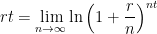
Since
![rt = \displaystyle \ln \left[ \lim_{n \to \infty} \left(1 + \frac{r}{n} \right)^{nt} \right]](https://s0.wp.com/latex.php?latex=rt+%3D+%5Cdisplaystyle+%5Cln+%5Cleft%5B+%5Clim_%7Bn+%5Cto+%5Cinfty%7D+%5Cleft%281+%2B+%5Cfrac%7Br%7D%7Bn%7D+%5Cright%29%5E%7Bnt%7D+%5Cright%5D&bg=ffffff&fg=000000&s=0&c=20201002)
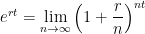
Finally, we multiply both sides by

(A second proof of this theorem, using L’Hopital’s Rule, will be presented in tomorrow’s post.)
This firmly established, at last, the connection between the continuous compound interest formula and the area under the hyperbola. I’ve noted that my students feel a certain sense of accomplishment after reaching this point of the exposition.
Different definitions of e (Part 8): Connecting the two definitions
In this series of posts, I consider how two different definitions of the number
- Algebra II/Precalculus: If
- Calculus: The number
These two definitions appear to be very, very different. One deals with making money. The other deals with the area under a hyperbola. Amazingly, these two definitions are related to each other. In this series of posts, I’ll discuss the connection between the two.
In yesterday’s post, I proved the following theorem, thus completing a long train of argument that began with the second definition of
Theorem. 
Proof #2. Let’s write the left-hand side as

Let’s take the natural logarithm of both sides:
![\ln L = \displaystyle \ln \left[ \lim_{h \to 0} \left( 1 + h \right)^{1/h} \right]](https://s0.wp.com/latex.php?latex=%5Cln+L+%3D+%5Cdisplaystyle+%5Cln+%5Cleft%5B+%5Clim_%7Bh+%5Cto+0%7D+%5Cleft%28+1+%2B+h+%5Cright%29%5E%7B1%2Fh%7D+%5Cright%5D&bg=ffffff&fg=000000&s=0&c=20201002)
Since


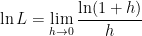
The right-hand side follows the indeterminate form
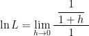


Therefore, the original limit is 

