In this series of posts, I’d like to describe what I tell my students on the very first day of Calculus I. On this first day, I try to set the table for the topics that will be discussed throughout the semester. I should emphasize that I don’t hold students immediately responsible for the content of this lecture. Instead, this introduction, which usually takes 30-45 minutes, depending on the questions I get, is meant to help my students see the forest for all of the trees. For example, when we start discussing somewhat dry topics like the definition of a continuous function and the Mean Value Theorem, I can always refer back to this initial lecture for why these concepts are ultimately important.
I’ve just told students that the topics in Calculus I build upon each other (unlike the topics of Precalculus), but that there are going to be two themes that run throughout the course:
- Approximating curved things by straight things, and
- Passing to limits
I then transition to applying these two themes to two different problems. Here’s the first.
Problem #1. A building on campus is 144 feet tall. A professor takes a particularly annoying student to the top of the building, and throws him (or her) off to his (or her) certain demise. (Usually I pick a student that I know and like as the one to throw off the building. This became a badge of honor over the years.) The distance that the student travels (in feet) after  seconds is
  . How fast is the student going when he (or she) hits the concrete sidewalk?
And then I ask my students how to solve this. Usually, they can come up with the first few ideas.
1. When the student hits the sidewalk and meet his/her demise? So we must solve  , so that
  . (And I make sure that they remember that this quadratic equation has two roots.) The solution
  is clearly extraneous, so the time elapsed until the student meets his/her demise is
  seconds.
2. How fast is the student going after seconds? Most students realize the inherent difficulty of this question because the student’s speed is increasing as he/she gets closer to the ground. Some students will volunteer the word “accelerate.”
At this point, I’ll volunteer that the changing speed is a curved thing. Back in pre-algebra, students were taught

under the assumption that the rate was constant. However, if the rate is changing, all bets are off.
Still, the question remains: how fast is the student moving after 3 seconds? How should we measure this? Usually, someone will suggest that we just divide  feet by seconds, for a rate of
  ft/sec. I then point out that this is an example of approximating a curved thing by a straight thing. The straight thing is the usual distance-rate-time formula, while the curved thing is the changing speed of the student as he/she falls. So the answer of ft/sec is not the correct answer, but it’s an approximate answer.
This leads to the next question: is this estimate too high or too low? Unequivocally, students answer “too low” since the student travels the slowest at the start of the fall and the fastest at the end of the fall. So since this interval of 3 seconds includes the slower speeds at the start of the fall, the answer of ft/sec will underestimate the speed at impact.
Which then leads to the next obvious question: How can we get a better approximation? I leave the question open-ended like this and take suggestions from the class. This often takes a while, and I’ll get a lot of creative (but bad) ideas. And that’s OK… the next step is hardly the most intuitive thing that immediately jumps to mind. I think that the process of keeping the answer unknown until someone volunteers the correct next step is worth it.
Eventually (though it might take a couple of minutes), somebody will suggest using a shorter time interval, like the distance traveled between  and
and  . We see that
  and
and  , and so the new approximation is
  ft/s. I store these two approximations ( ft/s with a time interval of seconds and
  ft/s with a time interval of
  second in a table on the side of the chalkboard. The values derived below are entered in the table as they’re found.
I then note that the previous approximation was ft/s, and then ask the class, “Do you think that ft/s will be a better or worse approximation than ft/s?” Invariably, they’ll say it’s a better approximation because the change in speed isn’t as great from to as from  to . I’ll then ask if they think that ft/s is too high or too low. Again, they’ll answer too low for the same reason as before.
Then I ask the obvious next question, “How do we find a better approximation?” The class typically responds something to the effect of, “Take a smaller interval.” I ask for a suggestion, and I’ll usually get something like  to . We see that
  ft/s and
  is still ft/s, so that the new approximation is
  ft/s. Students will volunteer that this should be better than the previous two approximations but still less than the correct answer.
Then I do it again: “How do we find a better approximation?” The class typically respond, “Take an even smaller interval.” I suggest  to . We see that
  ft/s (by this point, a calculator is certainly needed) and is still ft/s, so that the new approximation is
  ft/s. If we do it again with
  , we see that
  ft/s, for an approximation of
  ft/s.
ft/s.
I turn to the class and ask, “Have we found the right answer yet?” They’ll answer “No” in unison, but they’ll note that the approximations are probably pretty good right now. Astute students will notice that the approximations appear to be “leveling off” to some final value.
I’ll then tell the class that this is an example of passing to limits, the second theme of calculus. By making the time intervals smaller and smaller, we get better and better approximations to the true speed at impact. In the next post, I’ll describe how I informally introduce the concept of a limit with this example.
 between
  and
and  .
. . With ten rectangles, the approximation is
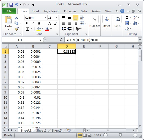
  . With one hundred rectangles (and Microsoft Excel), the approximation is
  . This last expression was found by evaluating
![0.01[ (0.01)^2 + (0.02)^2 + \dots + (0.99)^2 + 1^2]](https://s0.wp.com/latex.php?latex=0.01%5B+%280.01%29%5E2+%2B+%280.02%29%5E2+%2B+%5Cdots+%2B+%280.99%29%5E2+%2B+1%5E2%5D&bg=ffffff&fg=000000&s=0&c=20201002)
 . And so I’d feel comfortable showing my students the contents of this post. However, if I didn’t know for sure that my students had at least seen this formula, I probably would just ask them to guess the limiting answer without doing any of the algebra to follow.
 rectangles?” Without much difficulty, they’ll see that the rectangles have a common width of
  . The heights of the rectangles take a little more work to determine. I’ll usually work left to right. The left-most rectangle has right-most
  coordinate of
  . The next rectangle has a height of
  , and so we must evaluate
![\displaystyle \frac{1}{n} \left[ \frac{1^2}{n^2} + \frac{2^2}{n^2} + \dots + \frac{n^2}{n^2} \right]](https://s0.wp.com/latex.php?latex=%5Cdisplaystyle+%5Cfrac%7B1%7D%7Bn%7D+%5Cleft%5B+%5Cfrac%7B1%5E2%7D%7Bn%5E2%7D+%2B+%5Cfrac%7B2%5E2%7D%7Bn%5E2%7D+%2B+%5Cdots+%2B+%5Cfrac%7Bn%5E2%7D%7Bn%5E2%7D+%5Cright%5D&bg=ffffff&fg=000000&s=0&c=20201002) , or
, or![\displaystyle \frac{1}{n^3} \left[ 1^2 + 2^2 + \dots + n^2 \right]](https://s0.wp.com/latex.php?latex=%5Cdisplaystyle+%5Cfrac%7B1%7D%7Bn%5E3%7D+%5Cleft%5B+1%5E2+%2B+2%5E2+%2B+%5Cdots+%2B+n%5E2+%5Cright%5D&bg=ffffff&fg=000000&s=0&c=20201002)
 , or
, or  .
. ,
,  , and
, and  .
. is an example of a rational function, and so the horizontal asymptote can be immediately determined by dividing the leading coefficients of the numerator and denominator (since both have degree 2). We conclude that the limit is
  , and so that’s the area under the parabola.
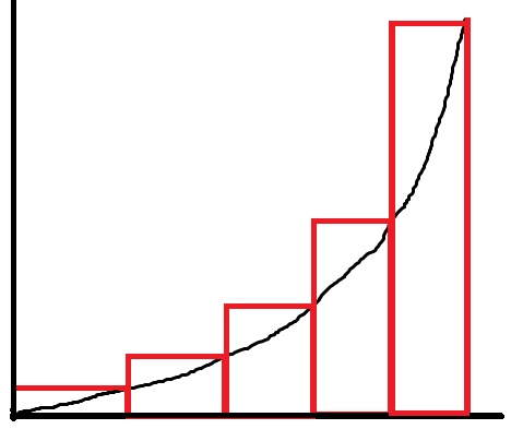
 , but the length takes a little bit more thought. And I make my students figure it out without me giving them the answer. Eventually, someone notices that the height is simply
  , so that the rightmost rectangle has an area of
  .
. . So the area is
  .
. . Students can easily see that this is a decent approximation to the area under the parabola, but it’s a bit too large.
![0.1 [ (0.1)^2 + (0.2)^2 + \dots + (0.9)^2 + 1^2] = 0.385](https://s0.wp.com/latex.php?latex=0.1+%5B+%280.1%29%5E2+%2B+%280.2%29%5E2+%2B+%5Cdots+%2B+%280.9%29%5E2+%2B+1%5E2%5D+%3D+0.385&bg=ffffff&fg=000000&s=0&c=20201002)
 rectangles, the class quickly sees that the sum of the rectangles is
![0.01 [ (0.01)^2 + (0.02)^2 + \dots + (0.99)^2 +( 1.00)^2] = 0.33835](https://s0.wp.com/latex.php?latex=0.01+%5B+%280.01%29%5E2+%2B+%280.02%29%5E2+%2B+%5Cdots+%2B+%280.99%29%5E2+%2B%28+1.00%29%5E2%5D+%3D+0.33835&bg=ffffff&fg=000000&s=0&c=20201002)
 seconds, the approximation is
  ft/s.
ft/s. seconds, the approximation is
  ft/s.
ft/s. seconds, the approximation is
  ft/s.
ft/s. seconds since dividing by zero is a no-no.
 and
and  ,
, ,
, is a small positive number. Let’s now simplify this fraction:


 .
. , then
  , matching the previous answer.
 , then
  , matching the previous answer.
 ft/s, which is the final answer.
 .
. between
  and
and  .
. and
and  are also decently large).
 and standard deviation
 , it doesn’t make much sense to show the full histogram; it suffices to have a maximum value around 5 or so.
 is small, then the normal approximation isn’t very good. I’ll say in words that there is a decent approximation under this limit, namely the Poisson distribution, but (for a class in statistics) I won’t say much more than that.
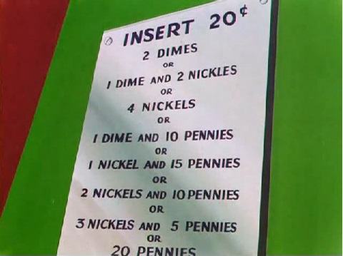
![\left[1 + x + x^2 + x^3 + x^4 + x^5 + \dots \right]](https://s0.wp.com/latex.php?latex=%5Cleft%5B1+%2B+x+%2B+x%5E2+%2B+x%5E3+%2B+x%5E4+%2B+x%5E5+%2B+%5Cdots+%5Cright%5D&bg=ffffff&fg=000000&s=0&c=20201002)
![\times \left[1 + x^5 + x^{10} + x^{15} + x^{20} + x^{25} + \dots \right]](https://s0.wp.com/latex.php?latex=%5Ctimes+%5Cleft%5B1+%2B+x%5E5+%2B+x%5E%7B10%7D+%2B+x%5E%7B15%7D+%2B+x%5E%7B20%7D+%2B+x%5E%7B25%7D+%2B+%5Cdots+%5Cright%5D&bg=ffffff&fg=000000&s=0&c=20201002)
![\times \left[1 + x^{10} + x^{20} + x^{30} + x^{40} + x^{50} + \dots \right]](https://s0.wp.com/latex.php?latex=%5Ctimes+%5Cleft%5B1+%2B+x%5E%7B10%7D+%2B+x%5E%7B20%7D+%2B+x%5E%7B30%7D+%2B+x%5E%7B40%7D+%2B+x%5E%7B50%7D+%2B+%5Cdots+%5Cright%5D&bg=ffffff&fg=000000&s=0&c=20201002)
![\times \left[1 + x^{25} + x^{50} + x^{75} + x^{100} + x^{125} + \dots \right]](https://s0.wp.com/latex.php?latex=%5Ctimes+%5Cleft%5B1+%2B+x%5E%7B25%7D+%2B+x%5E%7B50%7D+%2B+x%5E%7B75%7D+%2B+x%5E%7B100%7D+%2B+x%5E%7B125%7D+%2B+%5Cdots+%5Cright%5D&bg=ffffff&fg=000000&s=0&c=20201002)
 from the product of these four infinite series? I offer a thought bubble if you’d like to think about it before seeing the answer.


 : 15 pennies (15 cents) and 1 nickel (5 cents)
 ), we may write the infinite product as
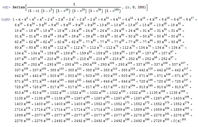
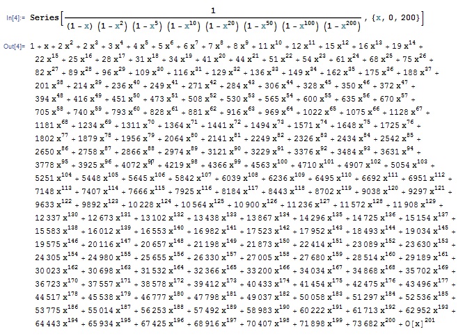
 — the coefficients provide the number of ways of expressing that many cents using pennies, nickels, dimes and quarters. This Taylor series can be computed with Mathematica:
 . The generating function for this sequence is
 , using the formula for an infinite geometric series.
 , the generating function is
 ,
, .
. if $0 \le n \le 10$ and
  for
for  . Then the generating function is
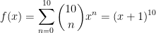 .
. denote the number of ways that
  . What about one dollar? Two dollars? I’ll provide the answer in tomorrow’s post.