I'm a Professor of Mathematics and a University Distinguished Teaching Professor at the University of North Texas. For eight years, I was co-director of Teach North Texas, UNT's program for preparing secondary teachers of mathematics and science.
Numerical integration is a standard topic in first-semester calculus. From time to time, I have received questions from students on various aspects of this topic, including:
Why is numerical integration necessary in the first place?
Where do these formulas come from (especially Simpson’s Rule)?
How can I do all of these formulas quickly?
Is there a reason why the Midpoint Rule is better than the Trapezoid Rule?
Is there a reason why both the Midpoint Rule and the Trapezoid Rule converge quadratically?
Is there a reason why Simpson’s Rule converges like the fourth power of the number of subintervals?
In this series, I hope to answer these questions. While these are standard questions in a introductory college course in numerical analysis, and full and rigorous proofs can be found on Wikipedia and Mathworld, I will approach these questions from the point of view of a bright student who is currently enrolled in calculus and hasn’t yet taken real analysis or numerical analysis.
In this post, we will perform an error analysis for the Trapezoid Rule
where is the number of subintervals and is the width of each subinterval, so that .
As noted above, a true exploration of error analysis requires the generalized mean-value theorem, which perhaps a bit much for a talented high school student learning about this technique for the first time. That said, the ideas behind the proof are accessible to high school students, using only ideas from the secondary curriculum (especially the Binomial Theorem), if we restrict our attention to the special case , where is a positive integer.
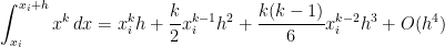
For this special case, the true area under the curve on the subinterval will be
In the above, the shorthand can be formally defined, but here we’ll just take it to mean “terms that have a factor of or higher that we’re too lazy to write out.” Since is supposed to be a small number, these terms will small in magnitude and thus can be safely ignored.
I wrote the above formula to include terms up to and including because I’ll need this later in this series of posts. For now, looking only at the Trapezoid Rule, it will suffice to write this integral as
.
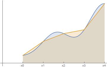
Using the Trapezoid Rule, we approximate as , using the width and the bases and of the trapezoid. Using the Binomial Theorem, this expands as
Once again, this is a little bit overkill for the present purposes, but we’ll need this formula later in this series of posts. Truncating somewhat earlier, we find that the Trapezoid Rule for this subinterval gives
Subtracting from the actual integral, the error in this approximation will be equal to
In other words, like the Midpoint Rule, both of the first two terms and cancel perfectly, leaving us with a local error on the order of .
We also recall, from the previous post in this series that the local error from the Midpoint Rule was . In other words, while both the Midpoint Rule and Trapezoid Rule have local errors on the order of , we expect the error in the Midpoint Rule to be about half of the error from the Trapezoid Rule.
Numerical integration is a standard topic in first-semester calculus. From time to time, I have received questions from students on various aspects of this topic, including:
Why is numerical integration necessary in the first place?
Where do these formulas come from (especially Simpson’s Rule)?
How can I do all of these formulas quickly?
Is there a reason why the Midpoint Rule is better than the Trapezoid Rule?
Is there a reason why both the Midpoint Rule and the Trapezoid Rule converge quadratically?
Is there a reason why Simpson’s Rule converges like the fourth power of the number of subintervals?
In this series, I hope to answer these questions. While these are standard questions in a introductory college course in numerical analysis, and full and rigorous proofs can be found on Wikipedia and Mathworld, I will approach these questions from the point of view of a bright student who is currently enrolled in calculus and hasn’t yet taken real analysis or numerical analysis.
In the previous post, we showed that the midpoint approximation of has error
In this post, we consider the global error when integrating on the interval instead of a subinterval . The logic for determining the global error is much the same as what we used earlier for the left-endpoint rule.
The total error when approximating will be the sum of the errors for the integrals over , , through . Therefore, the total error will be
.
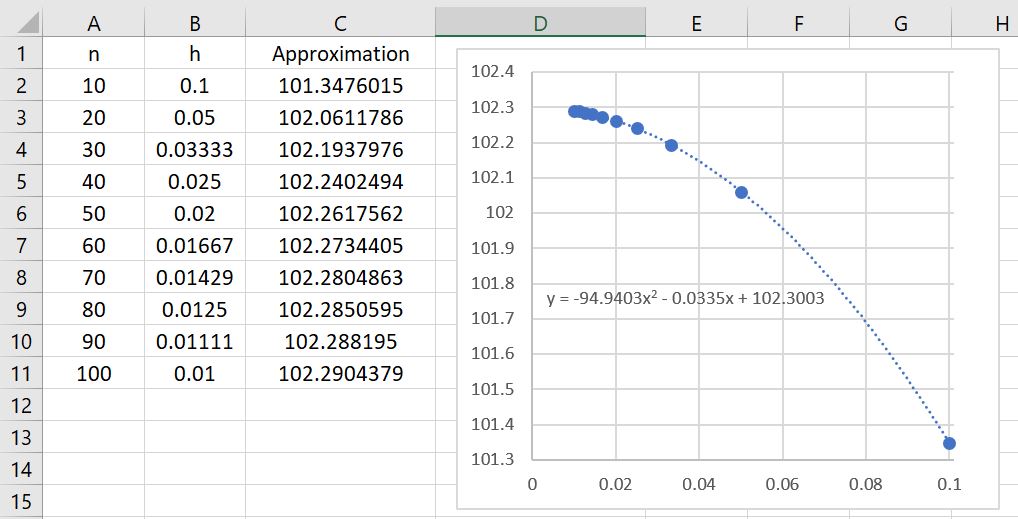
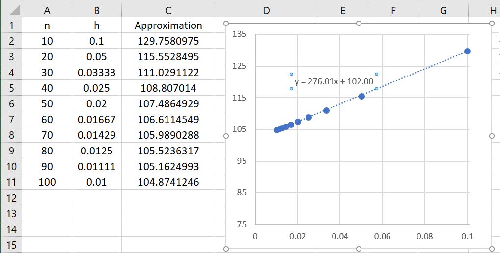
So that this formula doesn’t appear completely mystical, this actually matches the numerical observations that we made earlier. The figure below shows the left-endpoint approximations to for different numbers of subintervals. If we take and , then the error should be approximately equal to
,
which, as expected, is close to the actual error of .
Let , so that the error becomes
,
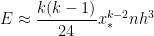
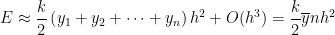
where is the average of the . Clearly, this average is somewhere between the smallest and the largest of the . Since is a continuous function, that means that there must be some value of between and — and therefore between and — so that by the Intermediate Value Theorem. We conclude that the error can be written as
,
Finally, since is the length of one subinterval, we see that is the total length of the interval . Therefore,
,
where the constant is determined by , , and . In other words, for the special case , we have established that the error from the Midpoint Rule is approximately quadratic in — without resorting to the generalized mean-value theorem and confirming the numerical observations we made earlier.
Numerical integration is a standard topic in first-semester calculus. From time to time, I have received questions from students on various aspects of this topic, including:
Why is numerical integration necessary in the first place?
Where do these formulas come from (especially Simpson’s Rule)?
How can I do all of these formulas quickly?
Is there a reason why the Midpoint Rule is better than the Trapezoid Rule?
Is there a reason why both the Midpoint Rule and the Trapezoid Rule converge quadratically?
Is there a reason why Simpson’s Rule converges like the fourth power of the number of subintervals?
In this series, I hope to answer these questions. While these are standard questions in a introductory college course in numerical analysis, and full and rigorous proofs can be found on Wikipedia and Mathworld, I will approach these questions from the point of view of a bright student who is currently enrolled in calculus and hasn’t yet taken real analysis or numerical analysis.
In this post, we will perform an error analysis for the Midpoint Rule
where is the number of subintervals and is the width of each subinterval, so that . Also, is the midpoint of the th subinterval.
As noted above, a true exploration of error analysis requires the generalized mean-value theorem, which perhaps a bit much for a talented high school student learning about this technique for the first time. That said, the ideas behind the proof are accessible to high school students, using only ideas from the secondary curriculum (especially the Binomial Theorem), if we restrict our attention to the special case , where is a positive integer.
For this special case, the true area under the curve on the subinterval will be
In the above, the shorthand can be formally defined, but here we’ll just take it to mean “terms that have a factor of or higher that we’re too lazy to write out.” Since is supposed to be a small number, these terms will small in magnitude and thus can be safely ignored.
I wrote the above formula to include terms up to and including because I’ll need this later in this series of posts. For now, looking only at the Midpoint Rule, it will suffice to write this integral as
.
Using the midpoint of the subinterval, the left-endpoint approximation of is . Using the Binomial Theorem, this expands as
Once again, this is a little bit overkill for the present purposes, but we’ll need this formula later in this series of posts. Truncating somewhat earlier, we find that the Midpoint Rule for this subinterval gives
Subtracting from the actual integral, the error in this approximation will be equal to
In other words, unlike the left-endpoint and right-endpoint approximations, both of the first two terms and cancel perfectly, leaving us with a local error on the order of .
The logic for determining the global error is much the same as what we used earlier for the left-endpoint rule.
The total error when approximating will be the sum of the errors for the integrals over , , through . Therefore, the total error will be
.
So that this formula doesn’t appear completely mystical, this actually matches the numerical observations that we made earlier. The figure below shows the left-endpoint approximations to for different numbers of subintervals. If we take and , then the error should be approximately equal to
,
which, as expected, is close to the actual error of .
Let , so that the error becomes
,
where is the average of the . Clearly, this average is somewhere between the smallest and the largest of the . Since is a continuous function, that means that there must be some value of between and — and therefore between and — so that by the Intermediate Value Theorem. We conclude that the error can be written as
,
Finally, since is the length of one subinterval, we see that is the total length of the interval . Therefore,
,
where the constant is determined by , , and . In other words, for the special case , we have established that the error from the Midpoint Rule is approximately quadratic in — without resorting to the generalized mean-value theorem and confirming the numerical observations we made earlier.
Numerical integration is a standard topic in first-semester calculus. From time to time, I have received questions from students on various aspects of this topic, including:
Why is numerical integration necessary in the first place?
Where do these formulas come from (especially Simpson’s Rule)?
How can I do all of these formulas quickly?
Is there a reason why the Midpoint Rule is better than the Trapezoid Rule?
Is there a reason why both the Midpoint Rule and the Trapezoid Rule converge quadratically?
Is there a reason why Simpson’s Rule converges like the fourth power of the number of subintervals?
In this series, I hope to answer these questions. While these are standard questions in a introductory college course in numerical analysis, and full and rigorous proofs can be found on Wikipedia and Mathworld, I will approach these questions from the point of view of a bright student who is currently enrolled in calculus and hasn’t yet taken real analysis or numerical analysis.
In the previous post in this series, we found that the local error of the right endpoint approximation to was equal to
.
We now consider the global error when integrating over the interval and not just a particular subinterval.
The total error when approximating will be the sum of the errors for the integrals over , , through . Therefore, the total error will be
.
So that this formula doesn’t appear completely mystical, this actually matches the numerical observations that we made earlier. The figure below shows the left-endpoint approximations to for different numbers of subintervals. If we take and , then the error should be approximately equal to
,
which, as expected, is close to the actual error of .
We now perform a more detailed analysis of the global error, which is almost a perfect copy-and-paste from the previous analysis. Let , so that the error becomes
,
where is the average of the . Clearly, this average is somewhere between the smallest and the largest of the . Since is a continuous function, that means that there must be some value of between and — and therefore between and — so that by the Intermediate Value Theorem. We conclude that the error can be written as
,
Finally, since is the length of one subinterval, we see that is the total length of the interval . Therefore,
,
where the constant is determined by , , and . In other words, for the special case , we have established that the error from the left-endpoint rule is approximately linear in — without resorting to the generalized mean-value theorem.
Numerical integration is a standard topic in first-semester calculus. From time to time, I have received questions from students on various aspects of this topic, including:
Why is numerical integration necessary in the first place?
Where do these formulas come from (especially Simpson’s Rule)?
How can I do all of these formulas quickly?
Is there a reason why the Midpoint Rule is better than the Trapezoid Rule?
Is there a reason why both the Midpoint Rule and the Trapezoid Rule converge quadratically?
Is there a reason why Simpson’s Rule converges like the fourth power of the number of subintervals?
In this series, I hope to answer these questions. While these are standard questions in a introductory college course in numerical analysis, and full and rigorous proofs can be found on Wikipedia and Mathworld, I will approach these questions from the point of view of a bright student who is currently enrolled in calculus and hasn’t yet taken real analysis or numerical analysis.
In this post, we will perform an error analysis for the right-endpoint rule
where is the number of subintervals and is the width of each subinterval, so that .
As noted above, a true exploration of error analysis requires the generalized mean-value theorem, which perhaps a bit much for a talented high school student learning about this technique for the first time. That said, the ideas behind the proof are accessible to high school students, using only ideas from the secondary curriculum, if we restrict our attention to the special case , where is a positive integer.
For this special case, the true area under the curve $f(x) = x^k$ on the subinterval will be
In the above, the shorthand can be formally defined, but here we’ll just take it to mean “terms that have a factor of or higher that we’re too lazy to write out.” Since is supposed to be a small number, these terms will be much smaller in magnitude that the terms that have or and thus can be safely ignored.
Using only the right-endpoint of the subinterval, the left-endpoint approximation of is
.
Subtracting, the error in this approximation will be equal to
Repeating the logic from the previous post in this series, this local error on , which is proportional to , generates a total error on that is proportional to . That is, the right-endpoint rule has an error that is approximately linear in , confirming the numerical observation that we made earlier in this series.
In my capstone class for future secondary math teachers, I ask my students to come up with ideas for engaging their students with different topics in the secondary mathematics curriculum. In other words, the point of the assignment was not to devise a full-blown lesson plan on this topic. Instead, I asked my students to think about three different ways of getting their students interested in the topic in the first place.
I plan to share some of the best of these ideas on this blog (after asking my students’ permission, of course).
This student submission comes from my former student Conner Dunn. His topic, from Geometry: finding the area of regular polygons.
How can technology be used to effectively engage students with this topic? Note: It’s not enough to say “such-and-such is a great website”; you need to explain in some detail why it’s a great website.
A good way to get students into the concept and see it’s real life use is to be given a realistic problem. The natural world doesn’t typically give you perfectly regular polygons, but we certainly like making them ourselves. Better yet, we can make regular polygons of a certain area knowing the methodology behind computing their areas. Using GeoGebra, I can challenge students to construct a regular polygon of an exact area using what they know about the use of equilateral triangles to compute area.
For example, let’s say I ask for a hexagon with an area of 12√3 square units. While there’s a few strategies of constructing a regular hexagon that Geometry students may know of, the strategy to shoot for here is to recognize this means we want a hexagon with a side length of 2 then construct the triangles. GeoGebra allows for students to use line segments and give them certain lengths, as well as construct angles using a virtual compass tool. Below is the solution to this example by constructing 6 equilateral triangles (each with an area of 2√3 square units) to form the regular hexagon.
How does this topic extend what your students should have learned in previous courses?
By the end of the unit, students will have learned the formula for finding the area of a polygon (A = (1/2) * a * p, with a being the apothem, and p being the perimeter). But a big part of this unit is how we derive the formula from the process in which we solve the area using this equilateral triangle method. From many previous courses, students will have learned both the order of operations and properties of equality in equations, and we use this previous knowledge to connect a geometric understanding of area to an algebraic one. For example, when we have the idea of multiplying the area of an equilateral triangle by the number of sides, n, in the polygon, we have A = (1/2) b * h * n. It is by the use of communitive property that students can rearrange the variables like this: A = (1/2)h*b * n. And then we conclude that the b*n reveals that the perimeter of the polygon plays a role in our equation. This may seem subtle, but students being fluent in this knowledge helps them work in their geometric understandings much easier.
How has this topic appeared in high culture (art, classical music, theatre, etc.)?
A big part of the method for understanding area of polygons is seeing how we can perfectly fit equilateral triangles inside of our polygons of choice. Perfectly fitting shapes into and around other shapes is something you see in mosaic art everywhere, particularly in Islamic architecture.
While mosaic artists are not necessarily calculating the areas of their art pieces (they might but I doubt it), a big part what makes these buildings so nice to look at is how the shapes fit with one another so nicely. This is an art that’s very intentional in its aesthetically pleasing aroma. This is something I think Geometry students can take to heart when confronting Geometry problems (a just as well with future courses). It’s the overlooked skill of literally connecting pieces together in order to get something we want. In the case of the Islamic architect, what we want is a pleasing building to look at, but math, of course, brings in more possible things to shoot for and equips us with plenty of pieces to (literally) connect together.

![\int_a^b f(x) \, dx \approx \frac{h}{2} \left[f(x_0) + 2f(x_1) + 2f(x_2) + \dots + 2f(x_{n-1}) +f(x_n) \right] \equiv T_n](https://s0.wp.com/latex.php?latex=%5Cint_a%5Eb+f%28x%29+%5C%2C+dx+%5Capprox+%5Cfrac%7Bh%7D%7B2%7D+%5Cleft%5Bf%28x_0%29+%2B+2f%28x_1%29+%2B+2f%28x_2%29+%2B+%5Cdots+%2B+2f%28x_%7Bn-1%7D%29+%2Bf%28x_n%29+%5Cright%5D+%5Cequiv+T_n&bg=ffffff&fg=000000&s=0&c=20201002)
 is the number of subintervals and
  is the width of each subinterval, so that
  .
.
 , where
  is a positive integer.
![[x_i, x_i +h]](https://s0.wp.com/latex.php?latex=%5Bx_i%2C+x_i+%2Bh%5D&bg=ffffff&fg=000000&s=0&c=20201002)
![\displaystyle \int_{x_i}^{x_i+h} x^k \, dx = \frac{1}{k+1} \left[ (x_i+h)^{k+1} - x_i^{k+1} \right]](https://s0.wp.com/latex.php?latex=%5Cdisplaystyle+%5Cint_%7Bx_i%7D%5E%7Bx_i%2Bh%7D+x%5Ek+%5C%2C+dx+%3D+%5Cfrac%7B1%7D%7Bk%2B1%7D+%5Cleft%5B+%28x_i%2Bh%29%5E%7Bk%2B1%7D+-+x_i%5E%7Bk%2B1%7D+%5Cright%5D&bg=ffffff&fg=000000&s=0&c=20201002)
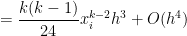
![= \displaystyle \frac{1}{k+1} \left[x_i^{k+1} + {k+1 \choose 1} x_i^k h + {k+1 \choose 2} x_i^{k-1} h^2 + {k+1 \choose 3} x_i^{k-2} h^3 + {k+1 \choose 4} x_i^{k-3} h^4+ {k+1 \choose 5} x_i^{k-4} h^5+ O(h^6) - x_i^{k+1} \right]](https://s0.wp.com/latex.php?latex=%3D+%5Cdisplaystyle+%5Cfrac%7B1%7D%7Bk%2B1%7D+%5Cleft%5Bx_i%5E%7Bk%2B1%7D+%2B+%7Bk%2B1+%5Cchoose+1%7D+x_i%5Ek+h+%2B+%7Bk%2B1+%5Cchoose+2%7D+x_i%5E%7Bk-1%7D+h%5E2+%2B+%7Bk%2B1+%5Cchoose+3%7D+x_i%5E%7Bk-2%7D+h%5E3+%2B+%7Bk%2B1+%5Cchoose+4%7D+x_i%5E%7Bk-3%7D+h%5E4%2B+%7Bk%2B1+%5Cchoose+5%7D+x_i%5E%7Bk-4%7D+h%5E5%2B+O%28h%5E6%29+-+x_i%5E%7Bk%2B1%7D+%5Cright%5D&bg=ffffff&fg=000000&s=0&c=20201002)

![+ \displaystyle \frac{(k+1)k(k-1)(k-2)(k-3)}{120} x_i^{k-4} h^5 \bigg] + O(h^6)](https://s0.wp.com/latex.php?latex=%2B+%5Cdisplaystyle+%5Cfrac%7B%28k%2B1%29k%28k-1%29%28k-2%29%28k-3%29%7D%7B120%7D+x_i%5E%7Bk-4%7D+h%5E5+%5Cbigg%5D+%2B+O%28h%5E6%29+&bg=ffffff&fg=000000&s=0&c=20201002)

 can be formally defined, but here we’ll just take it to mean “terms that have a factor of
  or higher that we’re too lazy to write out.” Since
  is supposed to be a small number, these terms will small in magnitude and thus can be safely ignored.
I wrote the above formula to include terms up to and including
is supposed to be a small number, these terms will small in magnitude and thus can be safely ignored.
I wrote the above formula to include terms up to and including  because I’ll need this later in this series of posts. For now, looking only at the Trapezoid Rule, it will suffice to write this integral as
 as
as ![\displaystyle \frac{h}{2} \left[x_i^k + (x_i + h)^k \right]](https://s0.wp.com/latex.php?latex=%5Cdisplaystyle+%5Cfrac%7Bh%7D%7B2%7D+%5Cleft%5Bx_i%5Ek+%2B+%28x_i+%2B+h%29%5Ek+%5Cright%5D&bg=ffffff&fg=000000&s=0&c=20201002) , using the width
, using the width  and
and  of the trapezoid. Using the Binomial Theorem, this expands as


 and
and  cancel perfectly, leaving us with a local error on the order of
  .
We also recall, from the previous post in this series that the local error from the Midpoint Rule was
.
We also recall, from the previous post in this series that the local error from the Midpoint Rule was  . In other words, while both the Midpoint Rule and Trapezoid Rule have local errors on the order of
  , we expect the error in the Midpoint Rule to be about half of the error from the Trapezoid Rule.
![[a,b]](https://s0.wp.com/latex.php?latex=%5Ba%2Cb%5D&bg=ffffff&fg=000000&s=0&c=20201002) instead of a subinterval
instead of a subinterval ![[x_i,x_i+h]](https://s0.wp.com/latex.php?latex=%5Bx_i%2Cx_i%2Bh%5D&bg=ffffff&fg=000000&s=0&c=20201002) . The logic for determining the global error is much the same as what we used earlier for the left-endpoint rule.
The total error when approximating
. The logic for determining the global error is much the same as what we used earlier for the left-endpoint rule.
The total error when approximating  will be the sum of the errors for the integrals over
 ![[x_0,x_1]](https://s0.wp.com/latex.php?latex=%5Bx_0%2Cx_1%5D&bg=ffffff&fg=000000&s=0&c=20201002) ,
, ![[x_1,x_2]](https://s0.wp.com/latex.php?latex=%5Bx_1%2Cx_2%5D&bg=ffffff&fg=000000&s=0&c=20201002) , through
, through ![[x_{n-1},x_n]](https://s0.wp.com/latex.php?latex=%5Bx_%7Bn-1%7D%2Cx_n%5D&bg=ffffff&fg=000000&s=0&c=20201002) . Therefore, the total error will be
. Therefore, the total error will be
 .
. for different numbers of subintervals. If we take
  and
and  , then the error should be approximately equal to
 ,
, .
.
 , so that the error becomes
 ,
, is the average of the
  . Clearly, this average is somewhere between the smallest and the largest of the
  is a continuous function, that means that there must be some value of
  between
  and
and  — and therefore between
  and
and  — so that
  by the Intermediate Value Theorem. We conclude that the error can be written as
 ,
, is the total length of the interval
 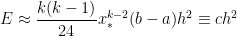 ,
, is determined by
  . In other words, for the special case
![\int_a^b f(x) \, dx \approx h \left[f(c_1) + f(c_2) + \dots + f(c_n) \right] \equiv M_n](https://s0.wp.com/latex.php?latex=%5Cint_a%5Eb+f%28x%29+%5C%2C+dx+%5Capprox+h+%5Cleft%5Bf%28c_1%29+%2B+f%28c_2%29+%2B+%5Cdots+%2B+f%28c_n%29+%5Cright%5D+%5Cequiv+M_n&bg=ffffff&fg=000000&s=0&c=20201002)
 is the midpoint of the
  th subinterval.

 . Using the Binomial Theorem, this expands as


 .
. will be the sum of the errors for the integrals over
  .
. ,
, .
.
 , so that the error becomes
 ,
, is the average of the
  is a continuous function, that means that there must be some value of
  and
and  — and therefore between
  by the Intermediate Value Theorem. We conclude that the error can be written as
 ,
, ,
,
![\int_a^b f(x) \, dx \approx h \left[f(x_1) + f(x_2) + \dots + f(x_n) \right] \equiv R_n](https://s0.wp.com/latex.php?latex=%5Cint_a%5Eb+f%28x%29+%5C%2C+dx+%5Capprox+h+%5Cleft%5Bf%28x_1%29+%2B+f%28x_2%29+%2B+%5Cdots+%2B+f%28x_n%29+%5Cright%5D+%5Cequiv+R_n&bg=ffffff&fg=000000&s=0&c=20201002)

![= \displaystyle \frac{1}{k+1} \left[x_i^{k+1} + {k+1 \choose 1} x_i^k h + {k+1 \choose 2} x_i^{k-1} h^2 + O(h^3) - x_i^{k+1} \right]](https://s0.wp.com/latex.php?latex=%3D+%5Cdisplaystyle+%5Cfrac%7B1%7D%7Bk%2B1%7D+%5Cleft%5Bx_i%5E%7Bk%2B1%7D+%2B+%7Bk%2B1+%5Cchoose+1%7D+x_i%5Ek+h+%2B+%7Bk%2B1+%5Cchoose+2%7D+x_i%5E%7Bk-1%7D+h%5E2+%2B+O%28h%5E3%29+-+x_i%5E%7Bk%2B1%7D+%5Cright%5D&bg=ffffff&fg=000000&s=0&c=20201002)
![= \displaystyle \frac{1}{k+1} \left[ (k+1) x_i^k h + \frac{(k+1)k}{2} x_i^{k-1} h^2 + O(h^3) \right]](https://s0.wp.com/latex.php?latex=%3D+%5Cdisplaystyle+%5Cfrac%7B1%7D%7Bk%2B1%7D+%5Cleft%5B+%28k%2B1%29+x_i%5Ek+h+%2B+%5Cfrac%7B%28k%2B1%29k%7D%7B2%7D+x_i%5E%7Bk-1%7D+h%5E2+%2B+O%28h%5E3%29+%5Cright%5D&bg=ffffff&fg=000000&s=0&c=20201002)

 and thus can be safely ignored.
 .
.
![[x_i, x_i+h]](https://s0.wp.com/latex.php?latex=%5Bx_i%2C+x_i%2Bh%5D&bg=ffffff&fg=000000&s=0&c=20201002) , which is proportional to
, which is proportional to  , generates a total error on


