I end this series about numerical integration by returning to the most common (if hidden) application of numerical integration in the secondary mathematics curriculum: finding the area under the normal curve. This is a critically important tool for problems in both probability and statistics; however, the antiderivative of 
In days of old, of course, students relied on tables in the back of the textbook to find areas under the bell curve, and I suppose that such tables are still being printed. For students with access to modern scientific calculators, of course, there’s no need for tables because this is a built-in function on many calculators. For the line of TI calculators, the command is normalcdf.
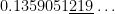
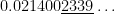
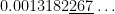
Unfortunately, it’s a sad (but not well-known) fact of life that the TI-83 and TI-84 calculators are not terribly accurate at computing these areas. For example:
TI-84:

Correct answer, with Mathematica:


TI-84: 
Correct answer, with Mathematica:
TI-84: 
Correct answer, with Mathematica:
TI-84: 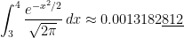
Correct answer, with Mathematica:
TI-84: 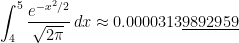
Correct answer, with Mathematica:

TI-84: 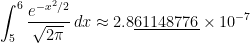
Correct answer, with Mathematica:

I don’t presume to know the proprietary algorithm used to implement normalcdf on TI-83 and TI-84 calculators. My honest if brutal assessment is that it’s probably not worth knowing: in the best case (when the endpoints are close to 0), the calculator provides an answer that is accurate to only 7 significant digits while presenting the illusion of a higher degree of accuracy. I can say that Simpson’s Rule with only 

For what it’s worth, I also looked at the accuracy of the NORMSDIST function in Microsoft Excel. This is much better, almost always producing answers that are accurate to 11 or 12 significant digits, which is all that can be realistically expected in floating-point double-precision arithmetic (in which numbers are usually stored accurate to 13 significant digits prior to any computations).
 . We obtained these approximations using only techniques within the reach of a talented high school student who has mastered Precalculus — especially the Binomial Theorem — and elementary techniques of integration.
 (and, by an easy extension, any polynomial), the formulas that we do obtain easily foreshadow the actual formulas found on Wikipedia or Mathworld or calculus textbooks, thus (hopefully) taking some of the mystery out of these formulas.
 ,
, is some number between
  and
and  . By comparison,
 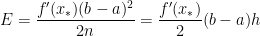 .
. .
. ,
, .
. .
. ,
, .
. ,
, .
. .
.
 or
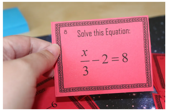
or  . Students should have learned that when they solve for the one-step equations (addition and subtract), whatever they do to one side of the equation, they need to make sure they add the same thing to the other side. For example, when they solve the equation
  . Therefore, x=8. Also, student should know that when they solve for the one-step equations (multiplication and division), they need to multiply both side by the reciprocal of the coefficient of the variable. For example, when they solve the equation
  for both sides, which is
  . Therefore,
  . Thus, when they learn to solve two-step equations, they need to combine these rules.
 has an error of
 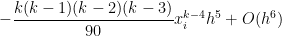 .
.![[a,b]](https://s0.wp.com/latex.php?latex=%5Ba%2Cb%5D&bg=ffffff&fg=000000&s=0&c=20201002) instead of a subinterval
instead of a subinterval ![[x_i,x_i+2h]](https://s0.wp.com/latex.php?latex=%5Bx_i%2Cx_i%2B2h%5D&bg=ffffff&fg=000000&s=0&c=20201002) .
The total error when approximating
.
The total error when approximating  will be the sum of the errors for the integrals over
 ![[x_0,x_2]](https://s0.wp.com/latex.php?latex=%5Bx_0%2Cx_2%5D&bg=ffffff&fg=000000&s=0&c=20201002) ,
, ![[x_2,x_4]](https://s0.wp.com/latex.php?latex=%5Bx_2%2Cx_4%5D&bg=ffffff&fg=000000&s=0&c=20201002) , through
, through ![[x_{n-2},x_n]](https://s0.wp.com/latex.php?latex=%5Bx_%7Bn-2%7D%2Cx_n%5D&bg=ffffff&fg=000000&s=0&c=20201002) . Therefore, the total error will be
. Therefore, the total error will be
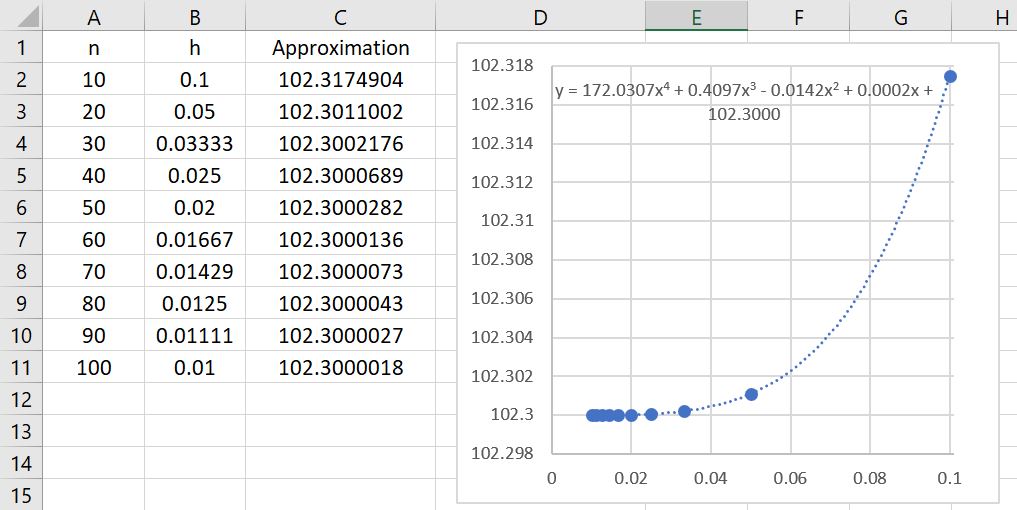
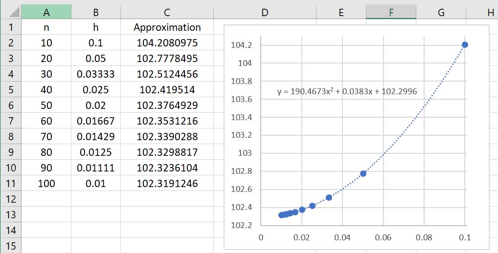
 for different numbers of subintervals. If we take
  and
and  , then the error should be approximately equal to
 ,
, .
.
 , so that the error becomes
 ,
, is the average of the
  . (We notice that there are only
  terms in this sum since we’re adding only the even terms.) Clearly, this average is somewhere between the smallest and the largest of the
  is a continuous function, that means that there must be some value of
  and
and  — and therefore between
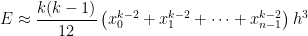
  by the Intermediate Value Theorem. We conclude that the error can be written as
 ,
, is the length of one subinterval, we see that
  is the total length of the interval
 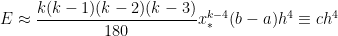 ,
, is determined by
  . In other words, for the special case
  + _HCl → _MnCl
 + _KCl + _Cl
![\int_a^b f(x) \, dx \approx \frac{h}{3} \left[f(x_0) + 4(x_1) + 2f(x_2) + \dots + 2f(x_{n-2}) + 4f(x_{n-1}) +f(x_n) \right] \equiv T_n](https://s0.wp.com/latex.php?latex=%5Cint_a%5Eb+f%28x%29+%5C%2C+dx+%5Capprox+%5Cfrac%7Bh%7D%7B3%7D+%5Cleft%5Bf%28x_0%29+%2B+4%28x_1%29+%2B+2f%28x_2%29+%2B+%5Cdots+%2B+2f%28x_%7Bn-2%7D%29+%2B+4f%28x_%7Bn-1%7D%29+%2Bf%28x_n%29+%5Cright%5D+%5Cequiv+T_n&bg=ffffff&fg=000000&s=0&c=20201002)
 is the number of subintervals (which has to be even) and
  is the width of each subinterval, so that
  .
.
 is a positive integer.
![[x_i, x_i +h]](https://s0.wp.com/latex.php?latex=%5Bx_i%2C+x_i+%2Bh%5D&bg=ffffff&fg=000000&s=0&c=20201002) will be
will be![\displaystyle \int_{x_i}^{x_i+h} x^k \, dx = \frac{1}{k+1} \left[ (x_i+h)^{k+1} - x_i^{k+1} \right]](https://s0.wp.com/latex.php?latex=%5Cdisplaystyle+%5Cint_%7Bx_i%7D%5E%7Bx_i%2Bh%7D+x%5Ek+%5C%2C+dx+%3D+%5Cfrac%7B1%7D%7Bk%2B1%7D+%5Cleft%5B+%28x_i%2Bh%29%5E%7Bk%2B1%7D+-+x_i%5E%7Bk%2B1%7D+%5Cright%5D&bg=ffffff&fg=000000&s=0&c=20201002)
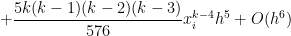
![= \displaystyle \frac{1}{k+1} \left[x_i^{k+1} + {k+1 \choose 1} x_i^k h + {k+1 \choose 2} x_i^{k-1} h^2 + {k+1 \choose 3} x_i^{k-2} h^3 + {k+1 \choose 4} x_i^{k-3} h^4+ {k+1 \choose 5} x_i^{k-4} h^5+ O(h^6) - x_i^{k+1} \right]](https://s0.wp.com/latex.php?latex=%3D+%5Cdisplaystyle+%5Cfrac%7B1%7D%7Bk%2B1%7D+%5Cleft%5Bx_i%5E%7Bk%2B1%7D+%2B+%7Bk%2B1+%5Cchoose+1%7D+x_i%5Ek+h+%2B+%7Bk%2B1+%5Cchoose+2%7D+x_i%5E%7Bk-1%7D+h%5E2+%2B+%7Bk%2B1+%5Cchoose+3%7D+x_i%5E%7Bk-2%7D+h%5E3+%2B+%7Bk%2B1+%5Cchoose+4%7D+x_i%5E%7Bk-3%7D+h%5E4%2B+%7Bk%2B1+%5Cchoose+5%7D+x_i%5E%7Bk-4%7D+h%5E5%2B+O%28h%5E6%29+-+x_i%5E%7Bk%2B1%7D+%5Cright%5D&bg=ffffff&fg=000000&s=0&c=20201002)

![+ \displaystyle \frac{(k+1)k(k-1)(k-2)(k-3)}{120} x_i^{k-4} h^5 \bigg] + O(h^6)](https://s0.wp.com/latex.php?latex=%2B+%5Cdisplaystyle+%5Cfrac%7B%28k%2B1%29k%28k-1%29%28k-2%29%28k-3%29%7D%7B120%7D+x_i%5E%7Bk-4%7D+h%5E5+%5Cbigg%5D+%2B+O%28h%5E6%29+&bg=ffffff&fg=000000&s=0&c=20201002)

 can be formally defined, but here we’ll just take it to mean “terms that have a factor of
  or higher that we’re too lazy to write out.” Since
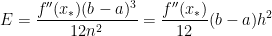
  relating the approximations from Simpson’s Rule, the Midpoint Rule, and the Trapezoid Rule. We now exploit this relationship to approximate
  . Earlier in this series, we found the Midpoint Rule approximation on this subinterval to be


 .
. subintervals, the Simpson’s Rule approximation of
  ,
,  , and
, and  — will be
  . Since
 ,
, ,
, ,
,
 .
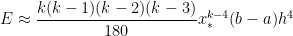
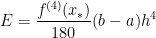
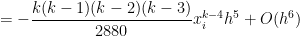
. perfectly match the first four terms of the exact value of the integral! Subtracting from the actual integral, the error in this approximation will be equal to

 , where
  and
and  , where only
 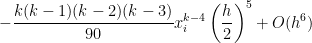 ,
, is the width of all of the
  , a vast improvement over both the Midpoint Rule and the Trapezoid Rule. This illustrates a general principle of numerical analysis: given two algorithms that are
  , an improved algorithm can typically be made by taking some linear combination of the two algorithms. Usually, the improvement will be to
  ; however, in this example, we magically obtained an improvement to

![[x_i,x_i+h]](https://s0.wp.com/latex.php?latex=%5Bx_i%2Cx_i%2Bh%5D&bg=ffffff&fg=000000&s=0&c=20201002) . The logic is almost a perfect copy-and-paste from the analysis used for the Midpoint Rule.
The total error when approximating
. The logic is almost a perfect copy-and-paste from the analysis used for the Midpoint Rule.
The total error when approximating ![[x_0,x_1]](https://s0.wp.com/latex.php?latex=%5Bx_0%2Cx_1%5D&bg=ffffff&fg=000000&s=0&c=20201002) ,
, ![[x_1,x_2]](https://s0.wp.com/latex.php?latex=%5Bx_1%2Cx_2%5D&bg=ffffff&fg=000000&s=0&c=20201002) , through
, through ![[x_{n-1},x_n]](https://s0.wp.com/latex.php?latex=%5Bx_%7Bn-1%7D%2Cx_n%5D&bg=ffffff&fg=000000&s=0&c=20201002) . Therefore, the total error will be
. Therefore, the total error will be
 .
. ,
, .
.
 , so that the error becomes
 ,
, is the average of the
  is a continuous function, that means that there must be some value of
  — and therefore between
  by the Intermediate Value Theorem. We conclude that the error can be written as
 ,
, ,
,