For years, various algorithms (derisively called “the computers” by sports commentators) have been used to rank college football teams. The source of derision is usually quite simple to explain: most of these algorithms are too hard to explain in layman’s terms, and therefore they are mocked.
For both its simplicity and its ability to provide reasonable rankings, my favorite algorithm is “Random Walker Rankings,” published at http://rwrankings.blogspot.com. Here is a concise description of this ranking system (quoted from http://rwrankings.blogspot.com/2003_12_01_archive.html):
We’ve all experienced befuddlement upon perusing the NCAA Division I-A college football
Bowl Championship Series (BCS) standings, because of the seemingly divine inspiration that must have been incorporated into their determination. The relatively small numbers of games between a large number of teams makes any ranking immediately suspect because of the dearth of head-to-head information. Perhaps you’ve even wondered if a bunch of monkeys could have ranked the football teams as well as the expert coaches and sportswriters polls and the complicated statistical ranking algorithms.We had these thoughts, so we set out to test this hypothesis, although with simulated monkeys (random walkers) rather than real ones.
Each of our simulated “monkeys” gets a single vote to cast for the “best” team in the nation, making their decisions based on only one simple guideline: They periodically look up the win-loss outcome of a single game played by their favorite team, and flip a weighted coin to determine whether to change their allegiance to the other team. In order to make this process even modestly reasonable, this random decision is made so that there is higher probability that the monkey’s allegiance and vote will go with the team that won the head-to-head contest. For instance, the weighting of the coin might be chosen so that 75% (say) of the time the monkey changes his vote to go with the winner of the game, meaning only a 25% chance of voting for the loser.
The monkey starts by voting for a randomly chosen team. Each monkey then meanders around a network which describes the collection of teams, randomly changing allegiance from one team to another along connections representing games played between the two teams that year. This network is graphically depicted in the figure here, with the monkeys—okay, technically one is a gorilla—not so happily lent to us by Ben Mucha (inset). It’s a simple process: if the outcome of the weighted coin flip indicates that he should be casting his vote for the opposing team, the monkey stops cheerleading for the old team and moves to the site in the network representing his new favorite team. While we let the monkeys change their minds over and over again—indeed, a single monkey voter will forever be changing his vote in this scheme—the percentage of votes cast for each football team quickly stabilizes. We thereby obtain rankings each week of the season and at the end of the season, based on the games played to that point of the season, by looking at the fraction of monkeys that vote for each team…
The virtue of this ranking system lies in its relative ease of explanation. Its performance is arguably on par with the expert polls and (typically more complicated) computer algorithms employed by the BCS. Can a bunch of monkeys rank football teams as well as the systems in use now? Perhaps they can.
Using this algorithm, here’s the current ranking of college football teams as of today. (With great pride, I note that Stanford is ranked #4.) These rankings certainly don’t exactly match the latest AP poll or BCS rankings, but they’re also still reasonable and defensible.

 for the area of a circle. However, they often tell me that they don’t remember a proof or justification for why this formula is true. And they certainly don’t remember a justification that would be appropriate for showing geometry students.
 is
is , or
, or 
 points on the circumference of the circle at every
  , and then draw the lines connecting these points and the center of the circle. Then have the students cut out these wedges and physically rearrange them as in the video. They should discover for themselves that the wedges approximately form a parallelogram, and they know how to find the area of a parallelogram.
 denotes a circular region with radius
  centered at the origin, then
 to
to  , while the angle varies from
  to
to  . Using the
  , we see that
![A = \displaystyle \int_0^{2\pi} \left[ \frac{r^2}{2} \right]_0^a \, d\theta](https://s0.wp.com/latex.php?latex=A+%3D+%5Cdisplaystyle+%5Cint_0%5E%7B2%5Cpi%7D+%5Cleft%5B+%5Cfrac%7Br%5E2%7D%7B2%7D+%5Cright%5D_0%5Ea+%5C%2C+d%5Ctheta&bg=ffffff&fg=000000&s=0&c=20201002)


![[0,2\pi]](https://s0.wp.com/latex.php?latex=%5B0%2C2%5Cpi%5D&bg=ffffff&fg=000000&s=0&c=20201002) and not
and not ![[0^o, 360^o]](https://s0.wp.com/latex.php?latex=%5B0%5Eo%2C+360%5Eo%5D&bg=ffffff&fg=000000&s=0&c=20201002) .
. may be viewed as the region between
  and
and  . These two functions intersect at
  and
and  . Therefore, the area of the circle is the integral of the difference of the two functions:
![A = \displaystyle \int_{-r}^r \left[g(x) - f(x) \right] \, dx= \displaystyle \int_{-r}^r 2 \sqrt{r^2 - x^2} \, dx](https://s0.wp.com/latex.php?latex=A+%3D+%5Cdisplaystyle+%5Cint_%7B-r%7D%5Er+%5Cleft%5Bg%28x%29+-+f%28x%29+%5Cright%5D+%5C%2C+dx%3D+%5Cdisplaystyle+%5Cint_%7B-r%7D%5Er+2+%5Csqrt%7Br%5E2+-+x%5E2%7D+%5C%2C+dx&bg=ffffff&fg=000000&s=0&c=20201002)
 and changing the range of integration to
  to
to  . Since
  , we find


![A = \displaystyle r^2 \left[ \theta + \frac{1}{2} \sin 2\theta \right]_{-\pi/2}^{\pi/2}](https://s0.wp.com/latex.php?latex=A+%3D+%5Cdisplaystyle+r%5E2+%5Cleft%5B+%5Ctheta+%2B+%5Cfrac%7B1%7D%7B2%7D+%5Csin+2%5Ctheta+%5Cright%5D_%7B-%5Cpi%2F2%7D%5E%7B%5Cpi%2F2%7D&bg=ffffff&fg=000000&s=0&c=20201002)
![A = \displaystyle r^2 \left[ \left( \displaystyle \frac{\pi}{2} + \frac{1}{2} \sin \pi \right) - \left( - \frac{\pi}{2} + \frac{1}{2} \sin (-\pi) \right) \right]](https://s0.wp.com/latex.php?latex=A+%3D+%5Cdisplaystyle+r%5E2+%5Cleft%5B+%5Cleft%28+%5Cdisplaystyle+%5Cfrac%7B%5Cpi%7D%7B2%7D+%2B+%5Cfrac%7B1%7D%7B2%7D+%5Csin+%5Cpi+%5Cright%29+-+%5Cleft%28+-+%5Cfrac%7B%5Cpi%7D%7B2%7D+%2B+%5Cfrac%7B1%7D%7B2%7D+%5Csin+%28-%5Cpi%29+%5Cright%29+%5Cright%5D&bg=ffffff&fg=000000&s=0&c=20201002)
![[-\pi/2,\pi/2]](https://s0.wp.com/latex.php?latex=%5B-%5Cpi%2F2%2C%5Cpi%2F2%5D&bg=ffffff&fg=000000&s=0&c=20201002) and not
and not ![[-90^o, 90^o]](https://s0.wp.com/latex.php?latex=%5B-90%5Eo%2C+90%5Eo%5D&bg=ffffff&fg=000000&s=0&c=20201002) .
.
 , a constant, then
  .
. and
and  are both differentiable, then
  .
. is a constant, then
  .
. , where
  is a nonnegative integer, then
  . This may be proved by at least two different techniques:
 is a polynomial, then
  . In other words, taking the derivative of a polynomial is easy.
 . Notice I’ve changed the variable from
  to
to  . Does this remind you of anything? (Students answer: Whoa… the circumference of a circle.)
 . Does this remind you of anything? (Students answer: the volume of a sphere.) What’s the derivative? Again,
  is just a constant. So
  . Does this remind you of anything? (Students answer: Whoa… the surface area of a sphere.)
 . In other words, imagine starting with a solid red disk of radius
  and then removing a solid white disk of radius
 . If this ring were to be “unpeeled” and flattened, it would approximately resemble a rectangle. The height of the rectangle would be
  , while the length of the rectangle would be the circumference of the circle. So

 , as above. Therefore, by the Fundamental Theorem of Calculus,

![A(r) - A(0) = \displaystyle \left[ \pi t^2 \right]_0^r](https://s0.wp.com/latex.php?latex=A%28r%29+-+A%280%29+%3D+%5Cdisplaystyle+%5Cleft%5B+%5Cpi+t%5E2+%5Cright%5D_0%5Er&bg=ffffff&fg=000000&s=0&c=20201002)

 is
is  , the area is
  and the perimeter is
  , which isn’t the derivative of
  . The reason this didn’t work is because the side length

 .
.
 or
or  .
. .
. is true, show
  is also true. This allows us to “carry” the fact that
  is true to the fact that
  is also true, and carry
  , etc., thus proving
  is always a factor of
  ).
). and
and  if
if  , proving that
  )
) if
if  )
)
 : The left-hand is simply
  , while the right-hand side is
  , which is also equal to
 ![\displaystyle \frac{(n+1)[(n+1)+1][2(n+1)+1]}{6} = \displaystyle \frac{(n+1)(n+2)(2n+3)}{6}](https://s0.wp.com/latex.php?latex=%5Cdisplaystyle+%5Cfrac%7B%28n%2B1%29%5B%28n%2B1%29%2B1%5D%5B2%28n%2B1%29%2B1%5D%7D%7B6%7D+%3D+%5Cdisplaystyle+%5Cfrac%7B%28n%2B1%29%28n%2B2%29%282n%2B3%29%7D%7B6%7D&bg=ffffff&fg=000000&s=0&c=20201002)

 . So we will substitute using the induction hypothesis, carrying the extra
 unnecessarily. Indeed, many early proofs by induction are simplified by factoring out terms whenever possible — in the example below,
  is factored on the third step — as opposed to multiplying them out. In my experience, proofs by induction often serve as a stringent test of students’ algebra skills as opposed to their skills in abstract reasoning.
![1^2 + 2^2 + \dots + (n-1)^2 + n^2 + (n+1)^2 = \displaystyle \frac{(n+1)[n(2n+1) + 6(n + 1)]}{6}](https://s0.wp.com/latex.php?latex=1%5E2+%2B+2%5E2+%2B+%5Cdots+%2B+%28n-1%29%5E2+%2B+n%5E2+%2B+%28n%2B1%29%5E2+%3D+%5Cdisplaystyle+%5Cfrac%7B%28n%2B1%29%5Bn%282n%2B1%29+%2B+6%28n+%2B+1%29%5D%7D%7B6%7D&bg=ffffff&fg=000000&s=0&c=20201002)


![\displaystyle \frac{[2(n+1)+1]^2}{8} = \displaystyle \frac{(2n+3)^2}{8}](https://s0.wp.com/latex.php?latex=%5Cdisplaystyle+%5Cfrac%7B%5B2%28n%2B1%29%2B1%5D%5E2%7D%7B8%7D+%3D+%5Cdisplaystyle+%5Cfrac%7B%282n%2B3%29%5E2%7D%7B8%7D&bg=ffffff&fg=000000&s=0&c=20201002)


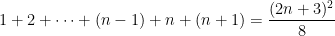
![\displaystyle \frac{[(2)(1) + 1]^2}{8} = \displaystyle \frac{9}{8}](https://s0.wp.com/latex.php?latex=%5Cdisplaystyle+%5Cfrac%7B%5B%282%29%281%29+%2B+1%5D%5E2%7D%7B8%7D+%3D+%5Cdisplaystyle+%5Cfrac%7B9%7D%7B8%7D&bg=ffffff&fg=000000&s=0&c=20201002) . So the base case is false.
. So the base case is false. degrees in a right angle,
  degrees in a straight angle, and a circle has
  degrees. They are introduced to
  and
and  right triangles. Fans of snowboarding even know the multiples of
  or even
  degrees.
 ,
,  ,
,  ,
,  , and multiples thereof.
 , but to visualize an angle of
  radians, they inevitably need to convert to degrees first. In his book
  and
and  look palatable.
 in a circle with radius

 and
and 
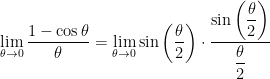
 makes the following computations from calculus a lot easier.
 , we replace
  to find
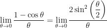


 and
and  — are needed to prove that
  and
and 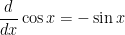 . Again, I won’t reinvent the wheel, but the proofs can be found
  floating around.
 is a first-grade problem, and students will use the number line (or their fingers) to reach the conclusion that
  . However, 6th graders taking Pre-Algebra are replacing the box with the variable
  , which is a proof! Having taken theorem-proof courses will allow you, the teacher, to explain why we can add a
  to both sides and it cancels out on one side and subtracts
  from the
  . Moreover, it explains that the minus sign just tells you which direction you are moving on the number line and why the word we came up with for that idea, subtraction, means “to take away, to go to the left.”
 irrational?”
 instead of
  ?”
?” , the probability that event
  happens or event
  happens, and
  , the chance that
  ,
,  ,
,  ,
,  or
or  .
. is incorrect.
 underlie some important concepts in calculus, including the proof of the intermediate value theorem, the rigorous definition of a definite integral, and the proof that the definite integral of the sum of two functions equals the sum of the two definite integrals.