In this series, I’m discussing how ideas from calculus and precalculus (with a touch of differential equations) can predict the precession in Mercury’s orbit and thus confirm Einstein’s theory of general relativity. The origins of this series came from a class project that I assigned to my Differential Equations students maybe 20 years ago.
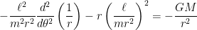
We previously showed that if the motion of a planet around the Sun is expressed in polar coordinates 
where 


the second equation arises since
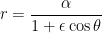
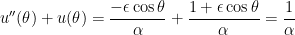
In the next few posts, we’ll discuss the solution of this initial-value problem. Today’s post would be appropriate for calculus students, which is confirming that
solves this initial-value problem, where 

As we’ve already seen in this series, this means that the orbit of the planet is a conic section — either a circle, ellipse, parabola, or hyperbola. Since the orbit of a planet is stable and 

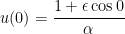
So, for a calculus student to verify that planets move in ellipses, one must check that
is a solution of the initial-value problem


The second line is easy to check:


The third line is also easy to check:
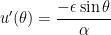
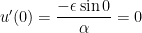
To check the first line, we first find 

so that
thus confirming that 
While the above calculations are well within the grasp of a good Calculus I student, I’ll be the first to admit that this solution is less than satisfying. We just mysteriously proposed a solution, seemingly out of thin air, and confirmed that it worked. In the next post, I’ll proposed a way that calculus students can be led to guess this solution. Then, we talk about finding the solution of this nonhomogeneous initial-value problem using standard techniques from differential equations.
 ,
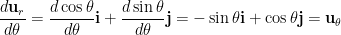
, and the acceleration
  are vectors. When written in polar coordinates, this becomes
![{\bf F} = m \displaystyle \left[ \frac{d^2r}{dt^2} - r \left( \frac{d\theta}{dt} \right)^2 \right] {\bf u}_r + m \left(r \frac{d^2 \theta}{d t^2} + 2 \frac{dr}{dt} \frac{d\theta}{dt} \right) {\bf u}_\theta](https://s0.wp.com/latex.php?latex=%7B%5Cbf+F%7D+%3D+m+%5Cdisplaystyle+%5Cleft%5B+%5Cfrac%7Bd%5E2r%7D%7Bdt%5E2%7D+-+r+%5Cleft%28+%5Cfrac%7Bd%5Ctheta%7D%7Bdt%7D+%5Cright%29%5E2+%5Cright%5D+%7B%5Cbf+u%7D_r+%2B+m+%5Cleft%28r+%5Cfrac%7Bd%5E2+%5Ctheta%7D%7Bd+t%5E2%7D+%2B+2+%5Cfrac%7Bdr%7D%7Bdt%7D+%5Cfrac%7Bd%5Ctheta%7D%7Bdt%7D+%5Cright%29+%7B%5Cbf+u%7D_%5Ctheta&bg=ffffff&fg=000000&s=0&c=20201002) ,
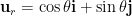
, is a unit vector pointing away from the origin and
  is a unit vector perpendicular to
  .
. ,
, is the mass of the sun,
  is the mass of the planet, and
  is the gravitational constant of the universe (which is a constant, no matter what
 ![m \displaystyle \left[ \frac{d^2r}{dt^2} - r \left( \frac{d\theta}{dt} \right)^2 \right] = \displaystyle -\frac{GMm}{r^2}](https://s0.wp.com/latex.php?latex=m+%5Cdisplaystyle+%5Cleft%5B+%5Cfrac%7Bd%5E2r%7D%7Bdt%5E2%7D+-+r+%5Cleft%28+%5Cfrac%7Bd%5Ctheta%7D%7Bdt%7D+%5Cright%29%5E2+%5Cright%5D+%3D+%5Cdisplaystyle+-%5Cfrac%7BGMm%7D%7Br%5E2%7D&bg=ffffff&fg=000000&s=0&c=20201002) ,
, .
. ,
, is a constant, and
 .
.


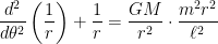
![\displaystyle \frac{\ell^2}{m^2 r^2} \left[ \frac{d^2}{d\theta^2} \left( \frac{1}{r} \right) + \frac{1}{r} \right] = \displaystyle \frac{GM}{r^2}](https://s0.wp.com/latex.php?latex=%5Cdisplaystyle++%5Cfrac%7B%5Cell%5E2%7D%7Bm%5E2+r%5E2%7D+%5Cleft%5B+%5Cfrac%7Bd%5E2%7D%7Bd%5Ctheta%5E2%7D+%5Cleft%28+%5Cfrac%7B1%7D%7Br%7D+%5Cright%29+%2B+%5Cfrac%7B1%7D%7Br%7D+%5Cright%5D++%3D+%5Cdisplaystyle+%5Cfrac%7BGM%7D%7Br%5E2%7D&bg=ffffff&fg=000000&s=0&c=20201002)
 .
. , we finally obtain the governing equation
 .
. as the constant on the right-hand side instead of just
  ,
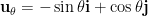
, are vectors. In usual rectangular coordinates, the acceleration vector would be expressed as
 ,
, and
and  directors are
  and
and  , and the unit vectors
  and
and  are perpendicular, pointing in the positive
  and positive
  directions.
 . This may be rewritten as
 ,
,
 .
.
 .
. .
. .
. , or a distance
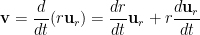

 .
.

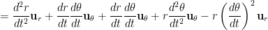
![= \displaystyle \left[ \frac{d^2r}{dt^2} - r \left(\frac{d\theta}{dt} \right)^2 \right] {\bf u}_r + \left[ 2\frac{dr}{dt} \frac{d\theta}{dt} + r \frac{d^2\theta}{dt^2} \right] {\bf u}_\theta](https://s0.wp.com/latex.php?latex=%3D+%5Cdisplaystyle+%5Cleft%5B+%5Cfrac%7Bd%5E2r%7D%7Bdt%5E2%7D+-++r+%5Cleft%28%5Cfrac%7Bd%5Ctheta%7D%7Bdt%7D+%5Cright%29%5E2+%5Cright%5D+%7B%5Cbf+u%7D_r+%2B+%5Cleft%5B+2%5Cfrac%7Bdr%7D%7Bdt%7D+%5Cfrac%7Bd%5Ctheta%7D%7Bdt%7D+%2B+r+%5Cfrac%7Bd%5E2%5Ctheta%7D%7Bdt%5E2%7D+%5Cright%5D+%7B%5Cbf+u%7D_%5Ctheta&bg=ffffff&fg=000000&s=0&c=20201002) .
. ,
, ;
; in a form that depends only on


 .
. .
.


![= \displaystyle \frac{\ell}{mr^2} \frac{d}{d\theta} \left[ \frac{dr}{dt} \right]](https://s0.wp.com/latex.php?latex=%3D+%5Cdisplaystyle+%5Cfrac%7B%5Cell%7D%7Bmr%5E2%7D+%5Cfrac%7Bd%7D%7Bd%5Ctheta%7D+%5Cleft%5B+%5Cfrac%7Bdr%7D%7Bdt%7D+%5Cright%5D&bg=ffffff&fg=000000&s=0&c=20201002)
![= \displaystyle \frac{\ell}{mr^2} \frac{d}{d\theta} \left[ - \frac{\ell}{m} \frac{d}{d\theta} \left( \frac{1}{r} \right) \right]](https://s0.wp.com/latex.php?latex=%3D+%5Cdisplaystyle+%5Cfrac%7B%5Cell%7D%7Bmr%5E2%7D+%5Cfrac%7Bd%7D%7Bd%5Ctheta%7D+%5Cleft%5B+-+%5Cfrac%7B%5Cell%7D%7Bm%7D+%5Cfrac%7Bd%7D%7Bd%5Ctheta%7D+%5Cleft%28+%5Cfrac%7B1%7D%7Br%7D+%5Cright%29+%5Cright%5D&bg=ffffff&fg=000000&s=0&c=20201002)
![= \displaystyle - \frac{\ell^2}{m^2r^2} \frac{d}{d\theta} \left[ \frac{d}{d\theta} \left( \frac{1}{r} \right) \right]](https://s0.wp.com/latex.php?latex=%3D+%5Cdisplaystyle+-+%5Cfrac%7B%5Cell%5E2%7D%7Bm%5E2r%5E2%7D+%5Cfrac%7Bd%7D%7Bd%5Ctheta%7D+%5Cleft%5B+%5Cfrac%7Bd%7D%7Bd%5Ctheta%7D+%5Cleft%28+%5Cfrac%7B1%7D%7Br%7D+%5Cright%29+%5Cright%5D&bg=ffffff&fg=000000&s=0&c=20201002)
 .
. .
. , or
, or .
. .
. .
. .
. . Then


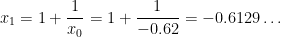
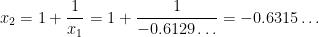
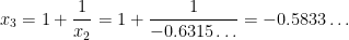
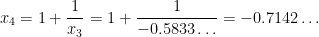
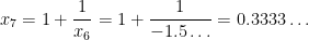
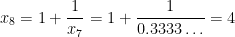
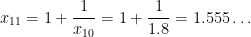
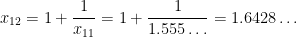
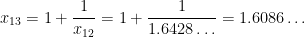
 into a calculator, then entering
  , and then repeatedly hitting the
  button.
 .
. .
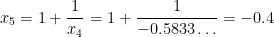
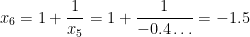
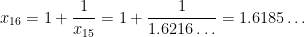
. . Unfortunately, if we start with a guess near this root, like
  , the sequence unexpectedly diverges from
  but eventually converges to the positive root
  :
:


 north,
  west, which is about 40 miles NNW of Spokane. (Images made by

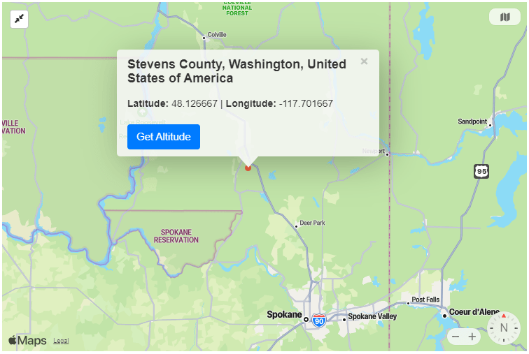
 north,
  west — which is indeed in Spokane — and then misconverted from decimal notation to minutes and seconds.

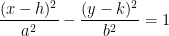
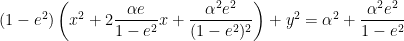
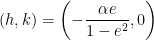
 . Furthermore, if
  , then this represents an ellipse with eccentricity
  whose major axis lies on the
  . Under this assumption,
  and
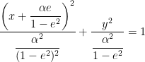
and  , so let me rewrite the previous equation in terms of
  :
:
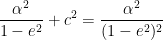
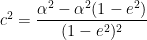
 ,
,
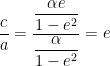
 from the center to the foci satisfies
 ,
,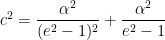
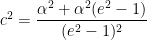


 , this means that the origin is, once again, one of the foci of the hyperbola.
 of the hyperbola is easily computed as
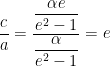 ,
,

 . With this substitution, the equation in rectangular coordinates simplifies to
 .
. , so that
  . Then the equation in rectangular coordinates simplifies to

 .
. ,
, to the left of the vertex. In other words, the origin is the focus of the parabola. (For what it’s worth, the directrix of the parabola would be the vertical line
  , located
  to the right of the vertex.)
 .
.


 so that
 .
. ,
, ,
, ,
, .
. ,
,


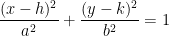
 . Therefore, since the foci of the ellipse are distance
  , or
, or  . That is, the origin is one focus of the ellipse. (For the little it’s worth, the other focus is located at
  .
. .
. . For this ellipse, the planet’s closest approach to the Sun occurs at
 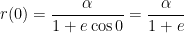 ,
, :
: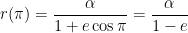 .
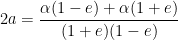
. of the major axis of the ellipse is the sum of these two distances:
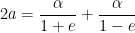

 .
. , we can also compute