Square roots and logarithms without a calculator (Part 12)

I recently came across the following computational trick: to estimate $\sqrt{b}$ , use

$\sqrt{b} \approx \displaystyle \frac{b+a}{2\sqrt{a}}$ ,

where $a$ is the closest perfect square to $b$ . For example,

$\sqrt{26} \approx \displaystyle \frac{26+25}{2\sqrt{25}} = 5.1$ .

I had not seen this trick before — at least stated in these terms — and I’m definitely not a fan of computational tricks without an explanation. In this case, the approximation is a straightforward consequence of a technique we teach in calculus. If $f(x) = (1+x)^n$ , then $f'(x) = n (1+x)^{n-1}$ , so that $f'(0) = n$ . Since $f(0) = 1$ , the equation of the tangent line to $f(x)$ at $x = 0$ is

$L(x) = f(0) + f'(0) \cdot (x-0) = 1 + nx$ .

The key observation is that, for $x \approx 0$ , the graph of $L(x)$ will be very close indeed to the graph of $f(x)$ . In Calculus I, this is sometimes called the linearization of $f$ at $x =a$ . In Calculus II, we observe that these are the first two terms in the Taylor series expansion of $f$ about $x = a$ .

For the problem at hand, if $n = 1/2$ , then

$\sqrt{1+x} \approx 1 + \displaystyle \frac{x}{2}$

if $x$ is close to zero. Therefore, if $a$ is a perfect square close to $b$ so that the relative difference $(b-a)/a$ is small, then

$\sqrt{b} = \sqrt{a + b - a}$

$= \sqrt{a} \sqrt{1 + \displaystyle \frac{b-a}{a}}$

$\approx \sqrt{a} \displaystyle \left(1 + \frac{b-a}{2a} \right)$

$= \sqrt{a} \displaystyle \left( \frac{2a + b-a}{2a} \right)$

$= \sqrt{a} \displaystyle \left( \frac{b+a}{2a} \right)$

$= \displaystyle \frac{b+a}{2\sqrt{a}}$ .

One more thought: All of the above might be a bit much to swallow for a talented but young student who has not yet learned calculus. So here’s another heuristic explanation that does not require calculus: if $a \approx b$ , then the geometric mean $\sqrt{ab}$ will be approximately equal to the arithmetic mean $(a+b)/2$ . That is,

$\sqrt{ab} \approx \displaystyle \frac{a+b}{2}$ ,

so that

$\sqrt{b} \approx \displaystyle \frac{a+b}{2\sqrt{a}}$ .

Engaging students: Geometric mean

In my capstone class for future secondary math teachers, I ask my students to come up with ideas for engaging their students with different topics in the secondary mathematics curriculum. In other words, the point of the assignment was not to devise a full-blown lesson plan on this topic. Instead, I asked my students to think about three different ways of getting their students interested in the topic in the first place.

I plan to share some of the best of these ideas on this blog (after asking my students’ permission, of course).

This student submission again comes from my former student Matthew Garza. His topic, from Geometry: the geometric mean.

How has this topic appeared in high culture?
Crockett Johnson was an artist, writer, and mathematician who worked as an art editor for McGraw-Hill in the 1920s. By the 1930s, he was making cartoons; in the 40s he was known for his “Barnaby” comic strips, which appeared in several American Newspapers. He wrote “Harold and the Purple Crayon” in 1955, which may be one his most famous works. In the 1960s he created a series of more than 100 paintings to honor of geometry and geometric mathematicians. Among them was this painting of a construction of the geometric mean of two numbers – line up the lengths and use that as the diameter of a circle, and draw a line from where the two lengths meet up to the circle. If the students know the Pythagorean theorem, they could try to prove that. Crockett Johnson also created a new construction of a regular septagon, using a compass and marked ruler (and trigonometric identities). I found another one of his mathematical paintings on the Smithsonian’s website, of a golden rectangle, and laid it over the geometric mean painting. It seems he included the golden ratio in his work, although I could not find anything verifying this. In general, Crockett Johnson is an interesting person, and that should help engage students.

Wikipedia page: https://en.wikipedia.org/wiki/Crockett_Johnson
Painting at Smithsonian: http://americanhistory.si.edu/collections/search/object/nmah_694664
Another Bio: https://divisbyzero.com/2016/03/23/a-geometry-theorem-looking-for-a-geometric-proof
Regular septagon proof: http://www.jstor.org/stable/3616804?seq=1#page_scan_tab_contents

How have different cultures throughout time used this topic in their society?
Finding much information on the history of the geometric mean is pretty difficult. Pythagoras seems to be generally credited for “discovering” the geometric mean, and the Greek mathematicians are famous for the three means – arithmetic, geometric, and harmonic. Although one not-necessarily credible source explained the word “geometry” comes from words meaning “land measurement.” From this, we can easily consider the task of land management – to find a square plot of land of equal area to a rectangular one, the side length of the square should be the geometric mean of the two sides of the rectangle. For this reason, I believe the geometric mean of at least two numbers must have been used as far back as math has been used for commerce; so pretty close to as far back as math has been used (I wouldn’t be surprised if Egyptians, or even Babylonians, were at least aware of such a relationship, whether or not a constructive proof existed).

http://hsm.stackexchange.com/questions/3057/what-is-the-history-of-the-meanings-behind-the-word-geometric

How has this topic appeared in the news?
Geometric mean is extremely useful for rates and values on varying scales. Rates are used as products – consider something like an investment with a varying return rate for each year. The regular arithmetic mean of the different rates would not give correct results – after one year at rate a, a quantity k becomes ak; after a second year at rate b, the original k is now bak. The yearly average, if taken arithmetically, gives [(a+b)²/4]k after 2 years; if the geometric mean is used, it gives (√ab)²k = abk, so it’s more appropriate. With regard to values on varying scales, it prevents a top-heavy average. Clearly, geometric mean is very useful, which is why finding news will work in a pinch, like if you forgot to plan. Just do a google news search for geometric mean and you find several articles. It’s mostly economic news. The following were not. Alternatively, a search in a scholarly database gives plenty of examples of geometric mean in action, although the technical writing may be difficult for students to get into for an engage.

Geometric mean to measure water quality: http://www.lajollalight.com/sd-beach-water-advisories-20161004-story.html
To measure general wellness of a nation: http://247wallst.com/healthcare-economy/2016/09/22/obesity-violence-helps-push-us-to-no-28-in-global-health-ratings
College sports stats: http://www.usatoday.com/story/sports/ncaaf/2016/10/11/sec-dominates-college-football-computer-composite-rankings/91910190/

My Favorite One-Liners: Part 77

In this series, I’m compiling some of the quips and one-liners that I’ll use with my students to hopefully make my lessons more memorable for them.

At the end of every semester, instructors are often asked “What do I need on the final to make a ___ in the course?”, where the desired course grade is given. (I’ve never done a survey, but A appears to be the most desired course grade, followed by C, D, and B.) Here’s the do-it-yourself algorithm that I tell my students, in which the final counts for 20% of the course average.

Let $F$ be the grade on the final exam (as I write a big F on the chalkboard). [groans] After all, final starts with $F$ , and it’s important to assign variable names that make sense.

Also, let $D$ be the up-to-date course average prior to the final. [more groans]

This gives us the course average. Just to be nice, let’s call that $A$ . [sighs of relief]

So $A = 0.2F + 0.8D$ .

More seriously, here’s a practical tip for students to determine what they need on the final to get a certain grade (hat tip to my friend Jeff Cagle for this idea). It’s based on the following principle:

If the average of $x_1, x_2, \dots x_n$ is $\overline{x}$ , then the average of $x_1 + c, x_2 + c, \dots, x_n + c$ is $\overline{x} + c$ . In other words, if you add a constant to a list of values, then the average changes by that constant.

As an application of this idea, let’s try to guess the average of $78, 82, 88, 90$ . A reasonable guess would be something like $85$ . So subtract $85$ from all four values, obtaining $-7, -3, 3, 5$ . The average of these four differences is $(-7-3+3+5)/4 = -0.5$ . Therefore, the average of the original four numbers is $85 + (-0.5) = 84.5$ .

So here’s a typical student question: “If my average right now is an $88$ , and the final is worth $20\%$ of my grade, then what do I need to get on the final to get a $90$ ?” Answer: The change in the average needs to be $+2$ , so the student needs to get a grade $+2/0.2 = +10$ points higher than his/her current average. So the grade on the final needs to be $88 + 10 = 98$ .

Seen another way, we’re solving the algebra problem

$88(0.8) + x(0.2) = 90$

Let me solve this in an unorthodox way:

$88(0.8) + x(0.2) = 88 + 2$

$88(0.8) + x(0.2) = 88(0.8+0.2) + 2$

$88(0.8) + x(0.2) = 88(0.8) + 88(0.2) + 2$

$x(0.2) = 88(0.2) + 2$

$x = \displaystyle \frac{88(0.2)}{0.2} + \frac{2}{0.2}$

$x = 88 + \displaystyle \frac{2}{0.2}$

This last line matches the solution found in the previous paragraph, $x = 88 + 10 = 98$ .

My Favorite One-Liners: Part 33

In this series, I’m compiling some of the quips and one-liners that I’ll use with my students to hopefully make my lessons more memorable for them.

Perhaps one of the more difficult things that I try to instill in my students is numeracy, or a sense of feeling if an answer to a calculation is plausible. As a initial step toward this goal, I’ll try to teach my students some basic pointers about whether an answer is even possible.

For example, when calculating a standard deviation, students have to compute $E(X)$ and $E(X^2)$ :

$E(X) = \sum x p(x) \qquad \hbox{or} \qquad E(X) = \int_a^b x f(x) \, dx$

$E(X^2) = \sum x^2 p(x) \qquad \hbox{or} \qquad E(X^2) = \int_a^b x^2 f(x) \, dx$

After these are computed — which could take some time — the variance is then calculated:

$\hbox{Var}(X) = E(X^2) - [E(X)]^2$ .

Finally, the standard deviation is found by taking the square root of the variance.

So, I’ll ask my students, what do you do if you calculate the variance and it’s negative, so that it’s impossible to take the square root? After a minute to students hemming and hawing, I’ll tell them emphatically what they should do:

It’s wrong… do it again.

The same principle applies when computing probabilities, which always have to be between 0 and 1. So, if ever a student computes a probability that’s either negative or else greater than 1, they can be assured that the answer is wrong and that there’s a mistake someplace in their computation that needs to be found.

My Favorite One-Liners: Part 15

In this series, I’m compiling some of the quips and one-liners that I’ll use with my students to hopefully make my lessons more memorable for them. Let me describe a one-liner that I’ll use when I want my class to figure out a pattern, thus developing a theorem by inductive logic rather than deductive logic.

Today’s one-liner is easily stated: “Gosh, I’ve seen that somewhere before.”

For example, In my statistics class, here’s the very first illustration that I show to demonstrate how to compute a standard deviation:

Find the standard deviation of the following data set: 1, 4, 6, 7, 8, 10.

The first step is finding the average:

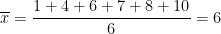$\overline{x} = \displaystyle \frac{1+4+6+7+8+10}{6} = 6$ .

We then find the deviations from average by subtracting 6 from all of the original data values:

Deviations from average = -5, -2, 0, 1, 2, 4

With these numbers, we can compute the standard deviation:

$s = \displaystyle \sqrt {\frac{ (-5)^2 + (-2)^2 + 0^2 + 1^2 + 2^2 + 4^2}{5} } = \sqrt{10}$ .

After asking if there are any questions of clarification about the nuts and bolts of this calculation, I’ll proceed to the next example:

Find the standard deviation of the following data set: 5, 8, 10, 11, 12, 14.

The first step is finding the average:

$\overline{x} = \displaystyle \frac{5+8+10+11+12+14}{6} = 10$ .

We then find the deviations from average by subtracting 10 from all of the original data values and then constructing the square root as before:

$s = \displaystyle \sqrt {\frac{ (-5)^2 + (-2)^2 + 0^2 + 1^2 + 2^2 + 4^2}{5} } = \sqrt{10}$ .

Then, in a loud obvious voice, I’ll declare, “Gosh, I’ve seen that somewhere before” and then wait a few seconds for the answer. Students can obviously see that the two answers are the same — which gets them thinking about why that happened.

Obviously, the two answers are the same. The real conceptual question that I want my students to figure out is why the two answers are same. Eventually, someone will come up with the correct answer — the second data set was made by adding 4 to all the values in the first data set, which may change the average but does not change how spread out the numbers are… so the standard deviation should be unchanged.

I love the “Gosh, I’ve seen that somewhere before” line after a couple of carefully chosen examples, as it cues my class that they really need to think a little harder than the dull and mechanical operations toward a deeper conceptual understanding of what’s really happening.

Deceiving with Statistics

I really enjoyed a recent Math With Bad Drawings post on how descriptive statistics can be used to deceive. For example:

See the rest of the post for similar picture for mean, median, mode, and variance (equivalent to standard deviation); I’ll be using these in my future statistics classes.

Why Not to Trust Statistics

Math with Bad Drawings has an excellent post on how the blind use of descriptive statistics can be deceptive. I’ll definitely be sharing a few these with my students. Here’s one of several examples; I recommend reading the whole thing.

The Inspection Paradox

From http://allendowney.blogspot.com/2015/08/the-inspection-paradox-is-everywhere.html:

Airlines complain that they are losing money because too many flights are nearly empty. At the same time passengers complain that flying is miserable because planes are too full. They could both be right. When a flight is nearly empty, only a few passengers enjoy the extra space. But when a flight is full, many passengers feel the crunch.

Once you notice the inspection paradox, you see it everywhere. Does it seem like you can never get a taxi when you need one? Part of the problem is that when there is a surplus of taxis, only a few customers enjoy it. When there is a shortage, many people feel the pain.

This article gives multiple examples (including computations) of the Inspection Paradox (also known as the Friendship Paradox), meaning that even the simple concept of “average” can be a little elusive. See also http://www.technologyreview.com/view/523566/how-the-friendship-paradox-makes-your-friends-better-than-you-are/

Averages and percentages

Source: http://www.xkcd.com/937/

Calculating course averages

And the end of every semester, instructors are often asked “What do I need on the final to make a ___ in the course?”, where the desired course grade is given. (I’ve never done a survey, but A appears to be the most desired course grade, followed by C, D, and B.) Here’s the do-it-yourself algorithm that I tell my students, in which the final counts for 20% of the course average.

Let $F$ be the grade on the final exam, and let $D$ be the up-to-date course average prior to the final. Then the course average is equal to $0.2F + 0.8D$ .

Somehow, students don’t seem comforted by this simple algebra.