About 15 years ago, when I was starting my career as an assistant professor, I was asked to write an article for Imagine magazine, which is targeted toward gifted students in grades 7-12, about what it’s like to be a math professor. While I would probably write something slightly different today (since my job responsibilities have shifted toward administration, academic advising, and the preparation of future secondary mathematics teachers), I think much of what I wrote still applies today.
Source: J. Quintanilla, “Beyond the Chalkboard: The Job of a Math Professor,” Imagine, Vol. 5, No. 4, p. 10 (March/April 1998).
One part of my job is deceptively simple to explain: I teach math to college students. Some people think I’ve got the easiest job in the world. I teach only two classes a semester for just six hours a week, and I have a flexible schedule with summers off. How cozy!
This view of my job is, of course, misleading. The hours I spend actually lecturing are only the tip of the iceberg. Delivering lectures that make sense and maintain students’ interest for a full hour takes considerable practice and effort. Meanwhile, I am constantly fine-tuning the curriculum, writing exams, and of course grading homework assignments — tasks which keep me working late on many nights. My most time-consuming project in recent months, however, has been to write eighty–and counting–letters of recommendation for former students.
My work with students outside the classroom includes one-on-one tutoring, guiding student research projects, advising students about possible majors and careers, and sometimes just lending an ear when someone’s had a rough day. As a professor I am a public figure on campus, and my current and former students come to me for counsel on a wide range of issues, many of which are only tangentially related to mathematics. I hope that through my words and counsel I am contributing to my students’ development as people as well as scholars.
In addition to lecturing, writing recommendations and counseling, I also have to produce original research. At my university, the quality of my teaching and my research will be weighted equally when I am evaluated for tenure in five years. The relative importance of teaching and research, however, varies from college to college. In general, small liberal arts colleges tend to emphasize teaching, while major universities want their professors to be primarily researchers.
When I started graduate school, I was introduced to my current field of research: applying ideas from probability theory to study theoretical problems in materials science. I have found that my research evolves over four stages: months of frustration, several days of sheer ecstasy when I’m overflowing with ideas, weeks of double-checking that my ideas actually make sense, and finally months of writing up my results for publication in scientific journals. I purposely work on three or four research projects
simultaneously, hoping that the cycle of each is slightly out of phase with the others. Though I work on my research all year, it gets my undivided attention during the summer when I’m not teaching.
Of the many aspects of this job, teaching is for me the most satisfying. I know that most of my students will not become professional mathematicians, so I incorporate “fun lectures” into the curriculum. These lectures illustrate how the mathematics we’re studying can be applied to fields of science. In my “Hunt for Red October” lecture, for example, I talk about applying trigonometry to linguistics, opera, and submarine detection; in my “Voyager 2” lecture, I describe how conic sections are used in planetary exploration. For my favorite fun lecture, I dress up in knickers, carry my golf clubs into class, and use calculus
to analyze the trajectory of golf balls. These lectures have become quite popular with my students, and I love to watch their eyes
light up when they’re excited about learning new things, such as how mathematics can be applied to real life.
Does this career sound appealing to you? If so, heed these words of warning: To become a successful professor, you have to really, really want this career. I am not a math professor for its financial rewards; friends of mine in industry earn salaries that are triple what I make. I don’t mind, and I’m not envious of them–I get to do what I love for a living, and I’m not starving. But this job isn’t for everyone. There are innumerable distractions and frustrations along the way that will derail aspiring professors who are not entirely focused on the goal.
For example, I always thought that I would be assured a job after graduation. In 1987, the National Science Foundation projected a shortfall of 675,000 scientists and engineers over the coming two decades. I was a high school senior in 1987, so I assumed I would be able to write my own ticket after earning a doctorate.
Time would show that this NSF projection, now derisively labeled “The Myth,” was amazingly inaccurate. There is currently an overproduction of Ph.D.s in mathematics, and the job market for aspiring math professors is tight. The unemployment rate for freshly-minted Ph.D.s in mathematics has hovered around 10% throughout the 1990s. A new Ph.D. can expect a nomadic
life — bouncing all over the country from one postdoctoral appointment to another — before finally landing a tenure-track position.
Faced with such daunting employment prospects, I braced myself for an unstable life in pursuit of my dream of becoming a professor. Even so, I must admit that getting avalanched by more than a hundred rejection letters was extremely disheartening. In the end, though, I was blessed with a tenure-track position straight out of grad school.
Like many jobs, the job of a math professor is frustrating at times and can feel overwhelming. But when it does, I think about the excited, curious students at a recent fun lecture and remind myself: I love this job!


and then start getting smaller. I’ll ask my students why this happens, and I’ll eventually get an explanation like


 .
. ,
, can be any number.
 .
. .
. .
. , which is so “flat” near $x=0$ that every single derivative of
  at
at  .
. is the
  coordinate at
  .
. is the slope of the curve at
  is a measure of the concavity of the curve at — you guessed it —
  is an even more subtle description of the curve… once again, at
  ,
,  ,
,  ,
,  , and
, and  .
. , and start differentiating. Remember that
  ,
,  ,
,  , and
, and  are constants.
 . Therefore, it must be that
  .
. , and so
  . Since
  .
. , and so
  . Since
  , or
, or  .
. , and so
  . Since
  , or
, or  .
. , and so
  . Since
  , or
, or  .
. .
. by
by  . Where did the
  , and so
 .
. by
by  . The number
  , and so
 .
. .
. and
and  .
. and
and  .
. .
. term has a coefficient involving the third derivative of
  and the last term is multiplied by
  .
. where have we seen those before? Oh yes, the
  ,
,  ,
,  ,
,  , and
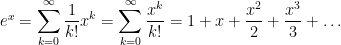
, and  is defined to be
  .
. notation:
 .
. are used over and over again in higher mathematics.
 A good working knowledge of Taylor series is necessary for computing series solutions of ordinary differential equations.
 are used over and over again. For example, the
 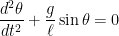 ,
, is the acceleration due to gravity and
  is the length of the pendulum. This differential equation cannot be solved exactly, and its solution is
  , so that the differential equation becomes
 ,
, term, we now have a second-order differential equation with constant coefficients, which can be solved in a straightforward manner using standard techniques from differential equations. If
  and
and  (i.e., the pendulum is pulled a small angle
  and is then released), the solution is
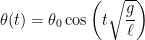 .
. , it doesn’t draw a unit circle, trace out an angle of
  in standard position, and find the
  coordinate of the terminal point. Instead, the calculator converts
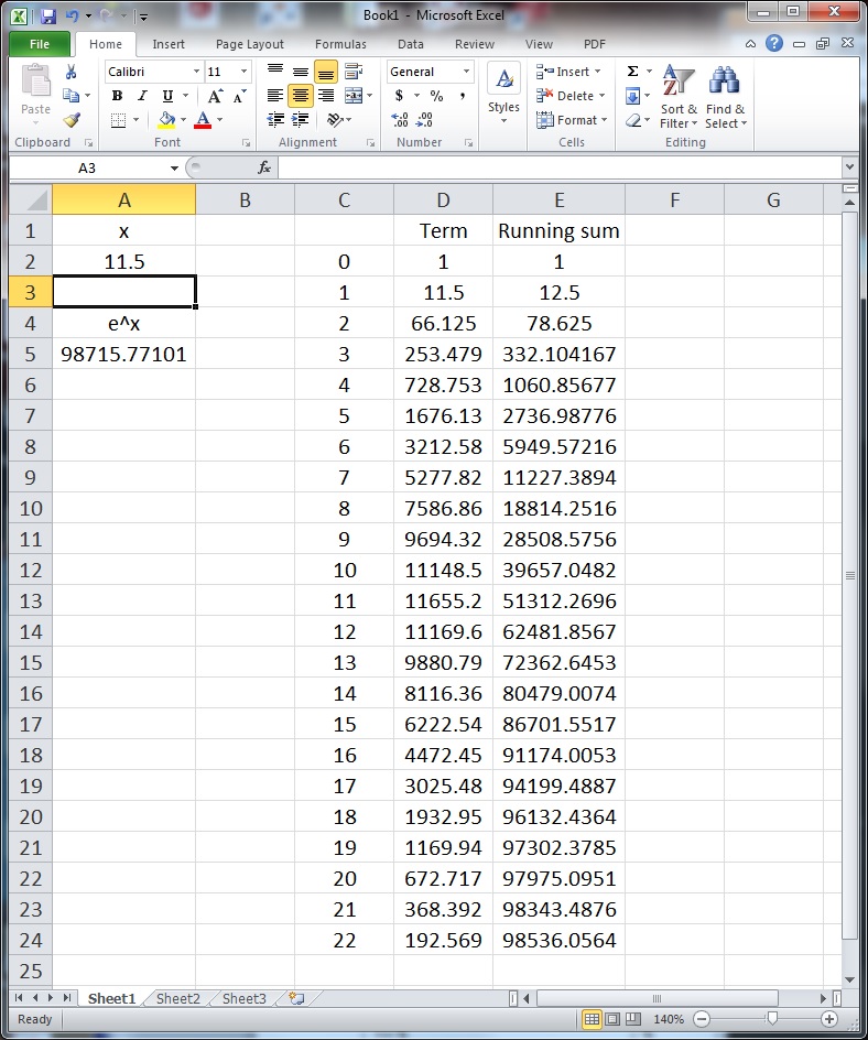
 , and (as I’ll discuss) the Maclaurin series for
  converges much faster than the Maclaurin series for
  at
at  .
. Height restriction)
 160 cm) The world’s largest hockey stick and puck are in Duncan, British Columbia. The stick is over 62 m in length and weighs almost 28,000 kg. Is your equipment legal?
 is shown)
 )
) ) While the child does this, the Magician calculates
  , writes the answer on a piece of paper, and turns the answer face down.

 , and there are indeed
  triangles in the figure.
 triangles created, then the
  degrees. So the sum of the measures of all of the angles must be
  degrees.
 degrees. Since there are
  degrees.
 degrees.
 , or
, or  .
. of two means, where at least one mean does not arise from a small sample, the Student t distribution must be employed. In particular, the number of degrees of freedom for the Student t distribution must be computed. Many textbooks suggest using
 is the standard error associated with the first average
  , where
  (if known) is the population standard deviation for
  and
and  is the number of samples that are averaged to find
  is employed.
 and
and  are similarly defined for the average
  .
. in the numerator is equal to
  . This is the square of the standard error
  associated with the difference
 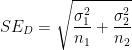 .
. ,
, .
.![df = \left( \displaystyle \frac{1}{n_1-1} \left[ \frac{SE_1^2}{SE_1^2 + SE_2^2}\right]^2 + \frac{1}{n_2-1} \left[ \frac{SE_2^2}{SE_1^2 + SE_2^2} \right]^2 \right)^{-1}](https://s0.wp.com/latex.php?latex=df+%3D+%5Cleft%28+%5Cdisplaystyle+%5Cfrac%7B1%7D%7Bn_1-1%7D+%5Cleft%5B+%5Cfrac%7BSE_1%5E2%7D%7BSE_1%5E2+%2B+SE_2%5E2%7D%5Cright%5D%5E2+%2B+%5Cfrac%7B1%7D%7Bn_2-1%7D+%5Cleft%5B+%5Cfrac%7BSE_2%5E2%7D%7BSE_1%5E2+%2B+SE_2%5E2%7D+%5Cright%5D%5E2+%5Cright%29%5E%7B-1%7D&bg=ffffff&fg=000000&s=0&c=20201002)
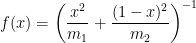
 and
and  , so that
![df = \left( \displaystyle \frac{1}{m_1} \left[ \frac{SE_1^2}{SE_1^2 + SE_2^2}\right]^2 + \frac{1}{m_2} \left[ \frac{SE_2^2}{SE_1^2 + SE_2^2} \right]^2 \right)^{-1}](https://s0.wp.com/latex.php?latex=df+%3D+%5Cleft%28+%5Cdisplaystyle+%5Cfrac%7B1%7D%7Bm_1%7D+%5Cleft%5B+%5Cfrac%7BSE_1%5E2%7D%7BSE_1%5E2+%2B+SE_2%5E2%7D%5Cright%5D%5E2+%2B+%5Cfrac%7B1%7D%7Bm_2%7D+%5Cleft%5B+%5Cfrac%7BSE_2%5E2%7D%7BSE_1%5E2+%2B+SE_2%5E2%7D+%5Cright%5D%5E2+%5Cright%29%5E%7B-1%7D&bg=ffffff&fg=000000&s=0&c=20201002)
 . All of these terms are nonnegative (and, in practice, they’re all positive), so that
  . Also, the numerator is no larger than the denominator, so that
  . Finally, we notice that
 .
. ,
, . Since
 ![[0,1]](https://s0.wp.com/latex.php?latex=%5B0%2C1%5D&bg=ffffff&fg=000000&s=0&c=20201002) , the absolute extrema can be found by checking the endpoints and the critical point(s).
, the absolute extrema can be found by checking the endpoints and the critical point(s). , then
  . On the other hand, if
  , then
  .
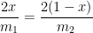
. :
:![f'(x) = -\left( \displaystyle \frac{x^2}{m_1} + \frac{(1-x)^2}{m_2} \right)^{-2} \left[ \displaystyle \frac{2x}{m_1} - \frac{2(1-x)}{m_2} \right] = 0](https://s0.wp.com/latex.php?latex=f%27%28x%29+%3D+-%5Cleft%28+%5Cdisplaystyle+%5Cfrac%7Bx%5E2%7D%7Bm_1%7D+%2B+%5Cfrac%7B%281-x%29%5E2%7D%7Bm_2%7D+%5Cright%29%5E%7B-2%7D+%5Cleft%5B+%5Cdisplaystyle+%5Cfrac%7B2x%7D%7Bm_1%7D+-+%5Cfrac%7B2%281-x%29%7D%7Bm_2%7D+%5Cright%5D+%3D+0&bg=ffffff&fg=000000&s=0&c=20201002)

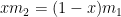


![f \left( \displaystyle \frac{m_1}{m_1+m_2} \right) = \left( \displaystyle \frac{1}{m_1} \frac{m_1^2}{(m_1+m_2)^2} + \frac{1}{m_2} \left[1-\frac{m_1}{m_1+m_2}\right]^2 \right)^{-1}](https://s0.wp.com/latex.php?latex=f+%5Cleft%28+%5Cdisplaystyle+%5Cfrac%7Bm_1%7D%7Bm_1%2Bm_2%7D+%5Cright%29+%3D+%5Cleft%28+%5Cdisplaystyle+%5Cfrac%7B1%7D%7Bm_1%7D+%5Cfrac%7Bm_1%5E2%7D%7B%28m_1%2Bm_2%29%5E2%7D+%2B+%5Cfrac%7B1%7D%7Bm_2%7D+%5Cleft%5B1-%5Cfrac%7Bm_1%7D%7Bm_1%2Bm_2%7D%5Cright%5D%5E2+%5Cright%29%5E%7B-1%7D&bg=ffffff&fg=000000&s=0&c=20201002)
![f \left( \displaystyle \frac{m_1}{m_1+m_2} \right) = \left( \displaystyle \frac{1}{m_1} \frac{m_1^2}{(m_1+m_2)^2} + \frac{1}{m_2} \left[\frac{m_2}{m_1+m_2}\right]^2 \right)^{-1}](https://s0.wp.com/latex.php?latex=f+%5Cleft%28+%5Cdisplaystyle+%5Cfrac%7Bm_1%7D%7Bm_1%2Bm_2%7D+%5Cright%29+%3D+%5Cleft%28+%5Cdisplaystyle+%5Cfrac%7B1%7D%7Bm_1%7D+%5Cfrac%7Bm_1%5E2%7D%7B%28m_1%2Bm_2%29%5E2%7D+%2B+%5Cfrac%7B1%7D%7Bm_2%7D+%5Cleft%5B%5Cfrac%7Bm_2%7D%7Bm_1%2Bm_2%7D%5Cright%5D%5E2+%5Cright%29%5E%7B-1%7D&bg=ffffff&fg=000000&s=0&c=20201002)


 and
and  , while the absolute maximum is equal to
  .
.
 is much smaller than
  ), then
  will be close to
  .
. ), then
  , but no larger.
 is the probability that the null hypothesis is correct due to dumb luck as opposed to a real effect (the alternative hypothesis). So if the significance level is really about
  and the experiment is repeated about 20 times, it wouldn’t be surprising for one of those experiments to falsely reject the null hypothesis.