Numerical integration is a standard topic in first-semester calculus. From time to time, I have received questions from students on various aspects of this topic, including:
- Why is numerical integration necessary in the first place?
- Where do these formulas come from (especially Simpson’s Rule)?
- How can I do all of these formulas quickly?
- Is there a reason why the Midpoint Rule is better than the Trapezoid Rule?
- Is there a reason why both the Midpoint Rule and the Trapezoid Rule converge quadratically?
- Is there a reason why Simpson’s Rule converges like the fourth power of the number of subintervals?
In this series, I hope to answer these questions. While these are standard questions in a introductory college course in numerical analysis, and full and rigorous proofs can be found on Wikipedia and Mathworld, I will approach these questions from the point of view of a bright student who is currently enrolled in calculus and hasn’t yet taken real analysis or numerical analysis.
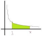
![]()
First, let’s talk about why numerical integration is necessary in the first place. Indeed, I can still remember a high school calculus teacher asking me this question nearly 20 years ago, and this question really got me thinking about what we’re collectively teaching in the secondary curriculum. Indeed, in a Calculus I course, it seems like every integral can be computed if only the proper trick is used. We teach students to search for these different tricks:
- Let
to find
.
- Let
to find
- Use integration by parts to find


In fact, we teach so many tricks that we may give the impression that every integral can be computed if only the proper trick is employed. Indeed, my university hosts an annual “Integration Bee” that challenges students to find the right technique(s) to evaluate some pretty tough integrals.
Unfortunately, not every integral can be solved in terms of a finite number of elementary functions (polynomials, rational functions, exponential functions, logarithms, trigonometric and inverse trigonometric functions). One function that is commonly known to many students which does not have an elementary antiderivative is 


cannot be found exactly, and so we ask students to either use a table in the back of the textbook or else use a function on their scientific calculators to find the answer.
Just for the fun of it, I went through my Ph.D. thesis and wrote down some of the integrals that I had to integrate numerically while in school. As an applied mathematician, I was initially stunned by the teacher’s innocent question because so much of my work would be utterly impossible if it wasn’t for numerical integration. Here are some of the easier ones:


![\displaystyle \int_0^{2R} e^{-sz} \exp \left[ -c \left( z \sqrt{4R^2-z^2} + 4R^2 \arcsin \frac{z}{2R} \right) \right] dz](https://s0.wp.com/latex.php?latex=%5Cdisplaystyle+%5Cint_0%5E%7B2R%7D+e%5E%7B-sz%7D+%5Cexp+%5Cleft%5B+-c+%5Cleft%28+z+%5Csqrt%7B4R%5E2-z%5E2%7D%C2%A0+%2B+4R%5E2+%5Carcsin+%5Cfrac%7Bz%7D%7B2R%7D+%5Cright%29+%5Cright%5D+dz&bg=ffffff&fg=000000&s=0&c=20201002)
![\displaystyle \int_0^d \exp \left[ -sz - \lambda \left(z - \frac{z^2}{4d} \right) \right] dz](https://s0.wp.com/latex.php?latex=%5Cdisplaystyle+%5Cint_0%5Ed+%5Cexp+%5Cleft%5B+-sz+-+%5Clambda+%5Cleft%28z+-+%5Cfrac%7Bz%5E2%7D%7B4d%7D+%5Cright%29+%5Cright%5D+dz&bg=ffffff&fg=000000&s=0&c=20201002)
![\displaystyle \int_d^{d \sqrt{2}} \exp \left[ -sz - \lambda \left( \frac{d (\pi+1)}{2} - d \arcsin \frac{d}{z} + \frac{z^2}{4d} - \sqrt{z^2-d^2} \right) \right] dz](https://s0.wp.com/latex.php?latex=%5Cdisplaystyle+%5Cint_d%5E%7Bd+%5Csqrt%7B2%7D%7D+%5Cexp+%5Cleft%5B+-sz+-+%5Clambda+%5Cleft%28+%5Cfrac%7Bd+%28%5Cpi%2B1%29%7D%7B2%7D+-+d+%5Carcsin+%5Cfrac%7Bd%7D%7Bz%7D+%2B+%5Cfrac%7Bz%5E2%7D%7B4d%7D+-+%5Csqrt%7Bz%5E2-d%5E2%7D+%5Cright%29+%5Cright%5D+dz&bg=ffffff&fg=000000&s=0&c=20201002)
![\displaystyle \int_0^\infty \exp \left[-sz - \eta \left(1 - e^{-cz/2} - \frac{cz}{4} e^{-cz/2} \right) \right] dz](https://s0.wp.com/latex.php?latex=%5Cdisplaystyle+%5Cint_0%5E%5Cinfty+%5Cexp+%5Cleft%5B-sz+-+%5Ceta+%5Cleft%281+-+e%5E%7B-cz%2F2%7D+-+%5Cfrac%7Bcz%7D%7B4%7D+e%5E%7B-cz%2F2%7D+%5Cright%29+%5Cright%5D+dz&bg=ffffff&fg=000000&s=0&c=20201002)

All this to say, there are plenty of integrals that arise from a real-world context that have a numerical answer but cannot be computed using the techniques commonly taught in the first-year calculus sequence.
 can be thought about in three different ways.
 .
. 2. We have the limits
 .
. . From this derivative,
  about
about  can be computed:
 to find
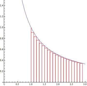
![[1,1.8]](https://s0.wp.com/latex.php?latex=%5B1%2C1.8%5D&bg=ffffff&fg=000000&s=0&c=20201002) and
and ![[1.8,2.6]](https://s0.wp.com/latex.php?latex=%5B1.8%2C2.6%5D&bg=ffffff&fg=000000&s=0&c=20201002) . (Because I need a good picture, I used Mathematica and not Microsoft Paint.)
. (Because I need a good picture, I used Mathematica and not Microsoft Paint.)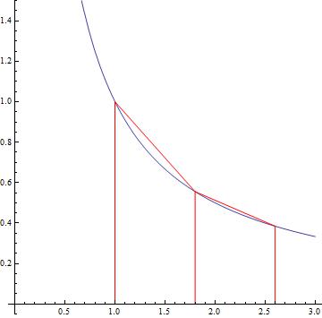
 . Furthermore, the bases of the first trapezoids have length
  and
and  , while the bases of the second trapezoid of length
  . Notice that the trapezoids extend above the hyperbola, so that
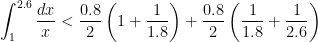

 , and so
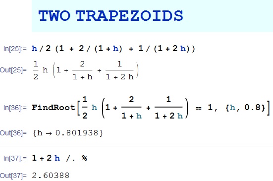
 is strictly less than
  . Can we do better? Sadly, with two equal-sized trapezoids, we can’t do much better. If the height of the trapezoids was
  and not
  , then the sum of the areas of the two trapezoids would be
 , thus establishing that
  .
.
 .
.
 .
.
 ranging from
  to
to  .
.
 to
to  . Therefore,
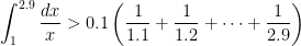

 is strictly greater than
  .
.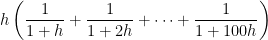

 . With 1000 rectangles, we can establish that
  .
. , but we’re not yet sure if the next digit is
  or
or  .
.