In this series, I’m exploring the following ancedote from the book Surely You’re Joking, Mr. Feynman!, which I read and re-read when I was young until I almost had the book memorized.
One day at Princeton I was sitting in the lounge and overheard some mathematicians talking about the series for e^x, which is 1 + x + x^2/2! + x^3/3! Each term you get by multiplying the preceding term by x and dividing by the next number. For example, to get the next term after x^4/4! you multiply that term by x and divide by 5. It’s very simple.
When I was a kid I was excited by series, and had played with this thing. I had computed e using that series, and had seen how quickly the new terms became very small.
I mumbled something about how it was easy to calculate e to any power using that series (you just substitute the power for x).
“Oh yeah?” they said. “Well, then what’s e to the 3.3?” said some joker—I think it was Tukey.
I say, “That’s easy. It’s 27.11.”
Tukey knows it isn’t so easy to compute all that in your head. “Hey! How’d you do that?”
Another guy says, “You know Feynman, he’s just faking it. It’s not really right.”
They go to get a table, and while they’re doing that, I put on a few more figures.: “27.1126,” I say.
They find it in the table. “It’s right! But how’d you do it!”
“I just summed the series.”
“Nobody can sum the series that fast. You must just happen to know that one. How about e to the 3?”
“Look,” I say. “It’s hard work! Only one a day!”
“Hah! It’s a fake!” they say, happily.
“All right,” I say, “It’s 20.085.”
They look in the book as I put a few more figures on. They’re all excited now, because I got another one right.
Here are these great mathematicians of the day, puzzled at how I can compute e to any power! One of them says, “He just can’t be substituting and summing—it’s too hard. There’s some trick. You couldn’t do just any old number like e to the 1.4.”
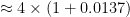
I say, “It’s hard work, but for you, OK. It’s 4.05.”
As they’re looking it up, I put on a few more digits and say, “And that’s the last one for the day!” and walk out.
What happened was this: I happened to know three numbers—the logarithm of 10 to the base e (needed to convert numbers from base 10 to base e), which is 2.3026 (so I knew that e to the 2.3 is very close to 10), and because of radioactivity (mean-life and half-life), I knew the log of 2 to the base e, which is.69315 (so I also knew that e to the.7 is nearly equal to 2). I also knew e (to the 1), which is 2. 71828.
The first number they gave me was e to the 3.3, which is e to the 2.3—ten—times e, or 27.18. While they were sweating about how I was doing it, I was correcting for the extra.0026—2.3026 is a little high.
I knew I couldn’t do another one; that was sheer luck. But then the guy said e to the 3: that’s e to the 2.3 times e to the.7, or ten times two. So I knew it was 20. something, and while they were worrying how I did it, I adjusted for the .693.
Now I was sure I couldn’t do another one, because the last one was again by sheer luck. But the guy said e to the 1.4, which is e to the.7 times itself. So all I had to do is fix up 4 a little bit!
They never did figure out how I did it.
My students invariably love this story; let’s take a look at the second calculation.
Feynman knew that  and
and  , so that
 .
.
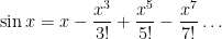
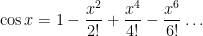
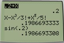
Therefore, again using the Taylor series expansion:


 .
.
Again, I have no idea how he put on a few more digits in his head (other than his sheer brilliance), as this would require knowing the values of  and
and  to six or seven digits as well as computing the next term in the Taylor series expansion:


$\approx 20 \times \left(1 + 0.0042677 + \frac{0.0042677^2}{2!} \right)$

This compares favorably with the actual answer,  .
.

 ,
, and the permissible values of
  are non-negative integers.
 .
. by
by  and then multiply both sides by
  :
: .
. .
. .
. .
. .
.

 .
. to any power. The terms get very small very quickly because of the factorials in the denominator, thus lending itself to the computation of
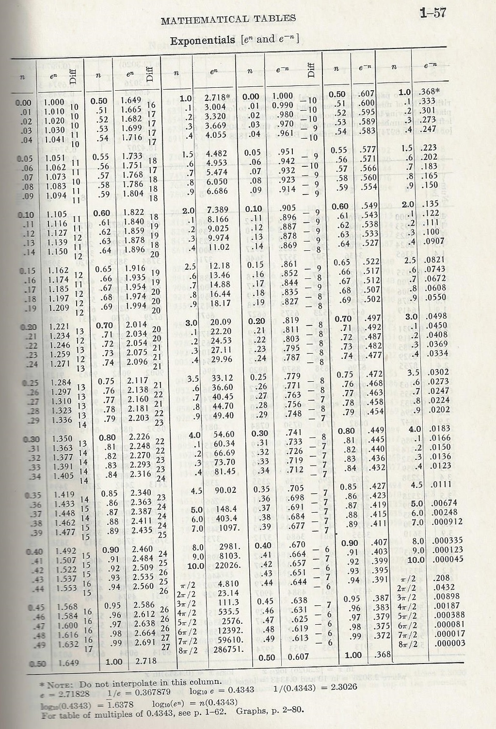
 . Somebody had computed all of these things (and plenty more) using the Taylor series, and they were compiled into a book and sold to mathematicians, scientists, and engineers.
 .
.

 . Therefore, we have
 .
.
 ,
, .
. , and so
 .
. .
. and
and  in my head took a minute or two:


 .
. and
and  . Therefore, I had the answer of
 .
.
 :
:
 .
. and diverges for
  . The boundary of
  , on the other hand, has to be checked separately for convergence.
 into the geometric series
 .
.
 .
. and identifying the coefficient for the term
  .
.
 has the form
  , where
  and
and  are differentiable functions so that
  and
and  . Therefore, we may rewrite this function using the Taylor series expansion of
  about
about  :
:![f(z) = \displaystyle \frac{1}{z-r} \left[ \frac{g(z)}{h(z)} \right]](https://s0.wp.com/latex.php?latex=f%28z%29+%3D+%5Cdisplaystyle+%5Cfrac%7B1%7D%7Bz-r%7D+%5Cleft%5B+%5Cfrac%7Bg%28z%29%7D%7Bh%28z%29%7D+%5Cright%5D&bg=ffffff&fg=000000&s=0&c=20201002)
![f(z) = \displaystyle \frac{1}{z-r} \left[ a_0 + a_1 (z-r) + a_2 (z-r)^2 + a_3 (z-r)^3 + \dots \right]](https://s0.wp.com/latex.php?latex=f%28z%29+%3D+%5Cdisplaystyle+%5Cfrac%7B1%7D%7Bz-r%7D+%5Cleft%5B+a_0+%2B+a_1+%28z-r%29+%2B+a_2+%28z-r%29%5E2+%2B+a_3+%28z-r%29%5E3+%2B+%5Cdots+%5Cright%5D&bg=ffffff&fg=000000&s=0&c=20201002)

![\displaystyle \lim_{z \to r} (z-r) f(z) = \displaystyle \lim_{z \to r} \left[ a_0 + a_1 (z-r) + a_2 (z-r)^2 + a_3 (z-r)^3 + \dots \right] = a_0](https://s0.wp.com/latex.php?latex=%5Cdisplaystyle+%5Clim_%7Bz+%5Cto+r%7D+%28z-r%29+f%28z%29+%3D+%5Cdisplaystyle+%5Clim_%7Bz+%5Cto+r%7D+%5Cleft%5B+a_0+%2B+a_1+%28z-r%29+%2B+a_2+%28z-r%29%5E2+%2B+a_3+%28z-r%29%5E3+%2B+%5Cdots+%5Cright%5D+%3D+a_0&bg=ffffff&fg=000000&s=0&c=20201002)
 . Notice that
 ,
, is the original denominator of
 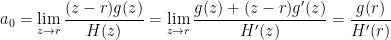 .
. and
and  , so that
  . Therefore, the residue at

 ,
, , or the constant term in the Taylor expansion of
 . Therefore, the residue at
  , matching the result found earlier.