I’m doing something that I should have done a long time ago: collecting a series of posts into one single post. The links below show my series on Lagrange points.
From Wikipedia, Lagrange points are points of equilibrium for small-mass objects under the gravitational influence of two massive orbiting bodies. There are five such points in the Sun-Earth system, called , , , , and .
The stable equilibrium points and are easiest to explain: they are the corners of equilateral triangles in the plane of Earth’s orbit. The points and are also equilibrium points, but they are unstable. Nevertheless, they have practical applications for spaceflight.
As we’ve seen, the positions of and can be found by numerically solving the fifth-order polynomial equations
and
,
respectively. In these equations, where is the mass of the Sun and is the mass of Earth. Also, is the distance from the Earth to or measured as a proportion of the distance from the Sun to Earth.
We’ve also seen that, for the Sun and Earth, , and numerically solving the above quintics yields for and for . In other words, and are approximately the same distance from Earth but in opposite directions.
There’s a good reason why the positive real roots of these two similar quintics are almost equal. We know that will be a lot closer to 0 than 1 because, for gravity to balance, the Lagrange points have to be a lot closer to Earth than the Sun. For this reason, the terms and will be a lot smaller than , and so those two terms can be safely ignored in a first-order approximation. Also, the terms and will be a lot smaller than , and so those two terms can also be safely ignored in a first-order approximation. Furthermore, since is also close to 0, the coefficient can be safely replaced by just .
Consequently, the solution of both quintic equations should be close to the solution of the cubic equation
,
which is straightforward to solve:
.
If , we obtain , which is indeed reasonably close to the actual solutions for and . Indeed, this may be used as the first approximation in Newton’s method to quickly numerically evaluate the actual solutions of the two quintic polynomials.
From Wikipedia, Lagrange points are points of equilibrium for small-mass objects under the gravitational influence of two massive orbiting bodies. There are five such points in the Sun-Earth system, called , , , , and .
The stable equilibrium points and are easiest to explain: they are the corners of equilateral triangles in the plane of Earth’s orbit. The points and are also equilibrium points, but they are unstable. Nevertheless, they have practical applications for spaceflight.
In this equation, is the mass of the Sun, is the mass of Earth, is the mass of the spacecraft, and is the distance from the Earth to measured as a proportion of the distance from the Sun to Earth. In other words, if the distance from the Sun to Earth is 1 unit, then the distance from the Earth to is units. The above equation is derived using principles from physics which are not elaborated upon here.
We notice that the coefficients of , , and are all positive, while the coefficients of , , and the constant term are all negative. Therefore, since there is only one change in sign, this equation has only one positive real root by Descartes’ Rule of Signs.
Since is orders of magnitude smaller than both and , this may safely approximated by
This yields a quintic equation that is hopeless to solve using standard techniques from Precalculus, but the root can be found graphically by seeing where the function crosses the axis (or, in this case, the axis):
As it turns out, the root is , so that is located of the distance from the Earth to the Sun in the direction away from the Sun.
From Wikipedia, Lagrange points are points of equilibrium for small-mass objects under the gravitational influence of two massive orbiting bodies. There are five such points in the Sun-Earth system, called , , , , and .
The stable equilibrium points and are easiest to explain: they are the corners of equilateral triangles in the plane of Earth’s orbit. The points and are also equilibrium points, but they are unstable. Nevertheless, they have practical applications for spaceflight.
In this equation, is the mass of the Sun, is the mass of Earth, is the mass of the spacecraft, and is the distance from the Earth to measured as a proportion of the distance from the Sun to . In other words, if the distance from the Sun to is 1 unit, then the distance from the Earth to is units. The above equation is derived using principles from physics which are not elaborated upon here.
We notice that the coefficients of , , and are all positive, while the coefficients of , , and the constant term are all negative. Therefore, since there is only one change in sign, this equation has only one positive real root by Descartes’ Rule of Signs.
Since is orders of magnitude smaller than both and , this may safely approximated by
.
Unfortunately, the unit is not as natural for Earth-bound observers as , the proportion of the distance of to Earth as a proportion of the distance from the Sun to Earth. Since is between the Sun and Earth, the distance from the Sun to Earth is units, so that . We then solve for in terms of (just like finding an inverse function):
.
Substituting into the above equation, we find an equation for :
Expanding, we find
Collecting like terms, we find
,
or
.
Again, this equation has only one positive real root since the original quintic in only had one positive real root. This new equation can be rewritten as
This yields a quintic equation that is hopeless to solve using standard techniques from Precalculus, but the root can be found graphically by seeing where the function crosses the axis (or, in this case, the axis):
As it turns out, the root is , so that is located of the distance from the Earth to the Sun in the direction of the Sun.
I recently read a terrific article in the American Mathematical Monthly about Lagrange points, which are (from Wikipedia) “points of equilibrium for small-mass objects under the gravitational influence of two massive orbiting bodies.” There are five such points in the Sun-Earth system, called , , , , and .
To describe these Lagrange points, I can do no better than the estimable Isaac Asimov. I quote from his essay “Colonizing the Heavens” from his book The Beginning and the End, which was published in 1977. I read the book over and over again as a boy in the mid-1980s. (Asimov’s essay originally concerned the Earth-Moon system; in the quote below, I changed the words to apply to the Sun-Earth system.)
Imagine the Sun at zenith, exactly overhead. Trace a line due eastward from the Sun down to the horizon. Two-thirds of the way along that line, one-third of the way up from the horizon, is one of those places. Trace another line westward away from the Sun down to the horizon. Two-thirds of the way along that line, one-third of the way up from the horizon, is another of those places.
Put an object in either place and it will form an equilateral triangle with the Sun and Earth…
What is so special about those places? Back in 1772, the astronomer Joseph Louis Lagrange showed that in those places any object remained stationary with respect to the Sun. As the Earth moved about the Sun, any object in either of those places would also move about the Sun in such a way as to keep perfect step with the Earth. The competing gravities of the Sun and Earth would keep it where it was. If anything happened to push it out of place it would promptly move back, wobbling back and forth a bit (“librating”) as it did so. The two places are called “Lagrangian points” or “libration points.”
Lagrange discovered five such places altogether, but three of them are of no importance since they don’t represent stable conditions. An object in those three places, once pushed out of place, would continue to drift outward and would never return.
The last paragraph of the above quote represents a rare failure of imagination by Asimov, who wrote prolifically about the future of spaceflight. Points and are indeed stable equilibria, and untold science fiction stories have placed spacecraft or colonies at these locations. (The rest of Asimov’s essay speculates about using these points in the Earth-Moon system for space colonization.) However, while the points and are unstable equilibria, they do have practical applications for spacecraft that can perform minor course corrections to stay in position. (The point is especially unstable to outside gravitational influences and thus seems unsuitable for spacecraft.) Again from Wikipedia,
Sun–Earth L1 is suited for making observations of the Sun–Earth system. Objects here are never shadowed by Earth or the Moon and, if observing Earth, always view the sunlit hemisphere… Solar and heliospheric missions currently located around L1 include the Solar and Heliospheric Observatory, Wind, Aditya-L1 Mission and the Advanced Composition Explorer. Planned missions include the Interstellar Mapping and Acceleration Probe(IMAP) and the NEO Surveyor.
Sun–Earth L2 is a good spot for space-based observatories. Because an object around L2 will maintain the same relative position with respect to the Sun and Earth, shielding and calibration are much simpler… The James Webb Space Telescope was positioned in a halo orbit about L2 on January 24, 2022.
Earth–Moon L1 allows comparatively easy access to Lunar and Earth orbits with minimal change in velocity and this has as an advantage to position a habitable space station intended to help transport cargo and personnel to the Moon and back. The SMART-1 Mission passed through the L1 Lagrangian Point on 11 November 2004 and passed into the area dominated by the Moon’s gravitational influence.
Earth–Moon L2 has been used for a communications satellite covering the Moon’s far side, for example, Queqiao, launched in 2018, and would be “an ideal location” for a propellant depot as part of the proposed depot-based space transportation architecture.
While the locations and are easy to describe, the precise locations of and are found by numerically solving a fifth-order polynomial equation. This was news to me when I read that article from the American Mathematical Monthly. While I had read years ago that finding the positions of the other three Lagrange points wasn’t simple, I did not realize that it was no more complicated that numerically finding the roots of a polynomial.
The above article from the American Mathematical Monthly concludes…
[t]he mathematical tools that Lagrange uses to arrive at a solution to this three-body problem lie entirely within the scope of modern courses in algebra, trigonometry, and first-semester calculus. But surely no ordinary person could have pursued the many extraordinarily complicated threads in his work to their ends, let alone woven them together into a magnificent solution to the problem as he has done. Lagrange noted in the introduction to his essay, “This research is really no more than for pure curiosity …” If only he could have watched on Christmas Day as the James Webb Space Telescope began its journey to the Lagrange point !
In this short series, we discuss the polynomial equations for finding and .
In this series, I’m discussing how ideas from calculus and precalculus (with a touch of differential equations) can predict the precession in Mercury’s orbit and thus confirm Einstein’s theory of general relativity. The origins of this series came from a class project that I assigned to my Differential Equations students maybe 20 years ago.
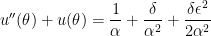
In the last few posts, I’ve used a standard technique from differential equations: to solve the th order homogeneous differential equation with constant coefficients
,
we first solve the characteristic equation
using techniques from Precalculus. The form of the roots determines the solutions of the differential equation.
While this is a standard technique from differential equations, the perspective I’m taking in this series is scaffolding the techniques used to predict the precession in a planet’s orbit using only techniques from Calculus and Precalculus. So let me discuss why the above technique works, assuming that the characteristic equation does not have repeated roots. (The repeated roots case is a little more complicated but is not needed for the present series of posts.)
We begin by guessing that the above differential equation has a solution of the form . Differentiating, we find , , etc. Therefore, the differential equation becomes
The last step does not “lose” any possible solutions for since can never be equal to . Therefore, solving the differential equation reduces to finding the roots of this polynomial, which can be done using standard techniques from Precalculus.
For example, one of the differential equations that we’ve encountered is . The characteristic equation is , which has roots . Therefore, two solutions to the differential equation are and , so that the general solution is
.
To write this in a more conventional way, we use Euler’s formula, so that
.
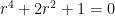
Likewise, in the previous post, we encountered the fourth-order differential equation . To find the roots of the characteristic equation, we factor:
.
Therefore, four solutions of this differential equation are , , , and , so that the general solution is
.
Using Euler’s formula as before, this can be rewritten as
In this series, I’m discussing how ideas from calculus and precalculus (with a touch of differential equations) can predict the precession in Mercury’s orbit and thus confirm Einstein’s theory of general relativity. The origins of this series came from a class project that I assigned to my Differential Equations students maybe 20 years ago.
We have shown that the motion of a planet around the Sun, expressed in polar coordinates with the Sun at the origin, under general relativity follows the initial-value problem
,
,
,
where , , , is the gravitational constant of the universe, is the mass of the planet, is the mass of the Sun, is the constant angular momentum of the planet, is the speed of light, and is the smallest distance of the planet from the Sun during its orbit (i.e., at perihelion).
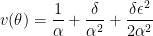
In this post, we will use the guesses
that arose from the technique/trick of reduction of order, where is some unknown function, to find the general solution of the differential equation
.
To do this, we will need to use the Product Rule for higher-order derivatives that was derived in the previous post:
and
.
In these formulas, Pascal’s triangle makes a somewhat surprising appearance; indeed, this pattern can be proven with mathematical induction.
We begin with . If , then
,
,
,
.
Substituting into the fourth-order differential equation, we find the differential equation becomes
The important observation is that the terms containing and cancelled each other. This new differential equation doesn’t look like much of an improvement over the original fourth-order differential equation, but we can make a key observation: if , then differentiating twice more trivially yields and . Said another way: if , then will be a solution of the original differential equation.
Integrating twice, we can find :
.
Therefore, a solution of the original differential equation will be
.
We now repeat the logic for :
.
Once again, a solution of this new differential equation will be , so that . Therefore, another solution of the original differential equation will be
.
Adding these provides the general solution of the differential equation:
.
Except for the order of the constants, this matches the solution that was presented earlier by using techniques taught in a proper course in differential equations.
In this series, I’m discussing how ideas from calculus and precalculus (with a touch of differential equations) can predict the precession in Mercury’s orbit and thus confirm Einstein’s theory of general relativity. The origins of this series came from a class project that I assigned to my Differential Equations students maybe 20 years ago.
We have shown that the motion of a planet around the Sun, expressed in polar coordinates with the Sun at the origin, under general relativity follows the initial-value problem
,
,
,
where , , , is the gravitational constant of the universe, is the mass of the planet, is the mass of the Sun, is the constant angular momentum of the planet, is the speed of light, and is the smallest distance of the planet from the Sun during its orbit (i.e., at perihelion).
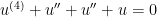
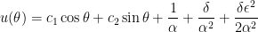
In the previous post, I used a standard technique from differential equations to find the general solution of
.
to be
.
However, as much as possible in this series, I want to take the perspective of a talented calculus student who has not yet taken differential equations — so that the conclusion above is far from obvious. How could this be reasonable coaxed out of such a student?
To begin, we observe that the characteristic equation is
,
or
.
Clearly this has the same roots as the simpler equation , which corresponds to the second-order differential equation . We’ve already seen that and are solutions of this differential equation; perhaps they might also be solutions of the more complicated differential equation also? The answer, of course, is yes:
and
.
The far trickier part is finding the two additional solutions. To find these, we use a standard trick/technique called reduction of order. In this technique, we guess that any additional solutions much have the form of either
,
where is some unknown function that we’re multiplying by the solutions we already have. We then substitute this into the differential equation to form a new differential equation for the unknown , which we can (hopefully) solve.
Doing this will require multiple applications of the Product Rule for differentiation. We already know that
.
We now differentiate again, using the Product Rule, to find :
.
We now differential twice more to find :
.
A good student may be able to guess the pattern for the next derivative:
.
In this way, Pascal’s triangle makes a somewhat surprising appearance; indeed, this pattern can be proven with mathematical induction.
In the next post, we’ll apply this to the solution of the fourth-order differential equation.
In this series, I’m discussing how ideas from calculus and precalculus (with a touch of differential equations) can predict the precession in Mercury’s orbit and thus confirm Einstein’s theory of general relativity. The origins of this series came from a class project that I assigned to my Differential Equations students maybe 20 years ago.
We have shown that the motion of a planet around the Sun, expressed in polar coordinates with the Sun at the origin, under general relativity follows the initial-value problem
,
,
,
where , , , is the gravitational constant of the universe, is the mass of the planet, is the mass of the Sun, is the constant angular momentum of the planet, is the speed of light, and is the smallest distance of the planet from the Sun during its orbit (i.e., at perihelion).
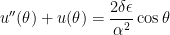
In the previous post, we derived the method of undetermined coefficients for the simplified differential equation
.
In this post, we consider the simplified differential equation if the right-hand side has only the fourth term,
.
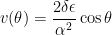
Let . Then satisfies the new differential equation . Since , we may substitute:
.
The characteristic equation of this homogeneous differential equation is , or . Therefore, and are both double roots of this quartic equation. Therefore, the general solution for is
.
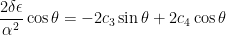
Substituting into the original differential equation will allow for the computation of and :
Matching coefficients, we see that and . Therefore,
is the general solution of the simplified differential equation. Setting , we find that
is one particular solution of this simplified differential equation. Not surprisingly, this matches the result is the method of undetermined coefficients had been blindly followed.
As we’ll see in a future post, the presence of this term is what predicts the precession of a planet’s orbit under general relativity.
In this series, I’m discussing how ideas from calculus and precalculus (with a touch of differential equations) can predict the precession in Mercury’s orbit and thus confirm Einstein’s theory of general relativity. The origins of this series came from a class project that I assigned to my Differential Equations students maybe 20 years ago.
We have shown that the motion of a planet around the Sun, expressed in polar coordinates with the Sun at the origin, under general relativity follows the initial-value problem
,
,
,
where , , , is the gravitational constant of the universe, is the mass of the planet, is the mass of the Sun, is the constant angular momentum of the planet, is the speed of light, and is the smallest distance of the planet from the Sun during its orbit (i.e., at perihelion).
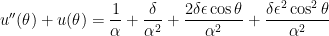
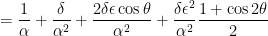
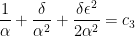
We now take the perspective of a student who is taking a first-semester course in differential equations. There are two standard techniques for solving a second-order non-homogeneous differential equations with constant coefficients. One of these is the method of constant coefficients. To use this technique, we first expand the right-hand side of the differential equation and then apply a power-reduction trigonometric identity:
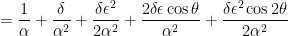
This is now in the form for using the method of undetermined coefficients. However, in this series, I’d like to take some time to explain why this technique actually works. To begin, we look at a simplified differential equation using only the first three terms on the right-hand side:
.
Let . Since is a constant, this function satisfies the simple differential equation . Since , we can substitute:
(We could have more easily said, “Take the derivative of both sides,” but we’ll be using a more complicated form of this technique in future posts.) The characteristic equation of this differential equation is . Factoring, we obtain , so that the three roots are and . Therefore, the general solution of this differential equation is
.
Notice that this matches the outcome of blindly using the method of undetermined coefficients without conceptually understanding why this technique works.
The constants and are determined by the initial conditions. To find , we observe
.
Therefore, the general solution of this simplified differential equation is
.
Furthermore, setting , we see that
is a particular solution to the differential equation
.
In the next couple of posts, we find the particular solutions associated with the other terms on the right-hand side.


 ,
,  , and
, and  .
.

 ,
, where
where  is the mass of the Sun and
  is the mass of Earth. Also,
  is the distance from the Earth to
  , and numerically solving the above quintics yields
  for
for  for
for  and
and  will be a lot smaller than
  , and so those two terms can be safely ignored in a first-order approximation. Also, the terms
  and
and  will be a lot smaller than
  , and so those two terms can also be safely ignored in a first-order approximation. Furthermore, since
  can be safely replaced by just
  .
.  ,
,

![t = \displaystyle \sqrt[3]{ \frac{\mu}{3} }](https://s0.wp.com/latex.php?latex=t+%3D+%5Cdisplaystyle+%5Csqrt%5B3%5D%7B+%5Cfrac%7B%5Cmu%7D%7B3%7D+%7D&bg=ffffff&fg=000000&s=0&c=20201002) .
. , we obtain
  , which is indeed reasonably close to the actual solutions for
 .
. is the mass of the spacecraft, and
  , and
, and  are all positive, while the coefficients of
  ,
,  .
. .
.
 ,
, ,
, and
and  , so that
 .
. axis (or, in this case, the
  axis):
 of the distance from the Earth to the Sun in the direction away from the Sun.
 .
. is the distance from the Earth to
  ,
,  , and
, and  are all positive, while the coefficients of
  ,
,  .
. units, so that
  . We then solve for


 .
.


 ,
, .
. .
. ,
, .
.
 , so that
  of the distance from the Earth to the Sun in the direction of the Sun.
 th order homogeneous differential equation with constant coefficients
 ,
,
 determines the solutions of the differential equation.
 . Differentiating, we find
  ,
,  , etc. Therefore, the differential equation becomes


 can never be equal to
  . Therefore, solving the differential equation reduces to finding the roots of this polynomial, which can be done using standard techniques from Precalculus.
 . The characteristic equation is
  , which has roots
  . Therefore, two solutions to the differential equation are
  and
and  , so that the general solution is
 .
. , so that


 .
. . To find the roots of the characteristic equation, we factor:


 .
. , and
, and  , so that the general solution is
 .
. .
. with the Sun at the origin, under general relativity follows the initial-value problem
  ,
, ,
, ,
, ,
,  ,
,  ,
,  is the gravitational constant of the universe,
  is the mass of the planet,
  is the mass of the Sun,
  is the constant angular momentum of the planet,
  is the speed of light, and
  is the smallest distance of the planet from the Sun during its orbit (i.e., at perihelion).
 is some unknown function, to find the general solution of the differential equation
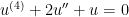 .
.
 .
. . If
. If  , then
 ,
, ,
, ,
, .
.


 and
and  cancelled each other. This new differential equation doesn’t look like much of an improvement over the original fourth-order differential equation, but we can make a key observation: if
  , then differentiating twice more trivially yields
  and
and  . Said another way: if

 .
. .
. :
:


 .
. , so that
  . Therefore, another solution of the original differential equation will be
 .
. .
. .
. ,
, .
. , which corresponds to the second-order differential equation
  . We’ve already seen that
  and
and  are solutions of this differential equation; perhaps they might also be solutions of the more complicated differential equation also? The answer, of course, is yes:
 .
. ,
, .
. :
:![(fg)'' = ( [fg]')' = (f'g)' + (fg')'](https://s0.wp.com/latex.php?latex=%28fg%29%27%27+%3D+%28+%5Bfg%5D%27%29%27+%3D+%28f%27g%29%27+%2B+%28fg%27%29%27&bg=ffffff&fg=000000&s=0&c=20201002)

 .
. :
:![(fg)''' = ( [fg]'')' = (f''g)' + 2(f'g')' + (fg'')'](https://s0.wp.com/latex.php?latex=%28fg%29%27%27%27+%3D+%28+%5Bfg%5D%27%27%29%27+%3D+%28f%27%27g%29%27+%2B+2%28f%27g%27%29%27+%2B++%28fg%27%27%29%27&bg=ffffff&fg=000000&s=0&c=20201002)

 .
.![(fg)^{(4)} = ( [fg]''')' = (f'''g)' + 3(f''g')' +3(f'g'')' + (fg''')'](https://s0.wp.com/latex.php?latex=%28fg%29%5E%7B%284%29%7D+%3D+%28+%5Bfg%5D%27%27%27%29%27+%3D+%28f%27%27%27g%29%27+%2B+3%28f%27%27g%27%29%27+%2B3%28f%27g%27%27%29%27+%2B+%28fg%27%27%27%29%27&bg=ffffff&fg=000000&s=0&c=20201002)

 .
. .
. .
. . Then
  satisfies the new differential equation
  . Since
  , we may substitute:
 . Therefore,
  and
and  are both double roots of this quartic equation. Therefore, the general solution for
  is
is .
. and
and  :
:

 and
and  . Therefore,
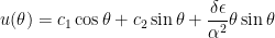
 , we find that
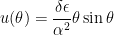
 term is what predicts the precession of a planet’s orbit under general relativity.
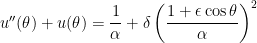 ,
,
 .
. . Since
  . Since
  , we can substitute:

 . Factoring, we obtain
  , so that the three roots are
  and
and  . Therefore, the general solution of this differential equation is
 .
. and
and  are determined by the initial conditions. To find
 .
. .
.
 .
.