In this series, I’m discussing how ideas from calculus and precalculus (with a touch of differential equations) can predict the precession in Mercury’s orbit and thus confirm Einstein’s theory of general relativity. The origins of this series came from a class project that I assigned to my Differential Equations students maybe 20 years ago.
We have shown that the motion of a planet around the Sun, expressed in polar coordinates 


where 


In this post, we will use the guesses

that arose from the technique/trick of reduction of order, where 
To do this, we will need to use the Product Rule for higher-order derivatives that was derived in the previous post:

and

In these formulas, Pascal’s triangle makes a somewhat surprising appearance; indeed, this pattern can be proven with mathematical induction.
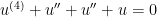
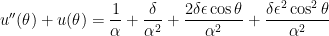
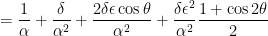
We begin with 


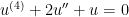
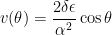
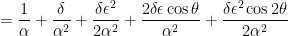
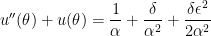
Substituting into the fourth-order differential equation, we find the differential equation becomes


The important observation is that the terms containing 


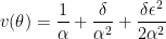
Integrating twice, we can find


Therefore, a solution of the original differential equation will be

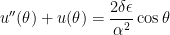
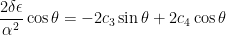
We now repeat the logic for 


Once again, a solution of this new differential equation will be 


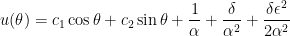
Adding these provides the general solution of the differential equation:

Except for the order of the constants, this matches the solution that was presented earlier by using techniques taught in a proper course in differential equations.
 .
. ,
, .
. , which corresponds to the second-order differential equation
  . We’ve already seen that
  and
and  are solutions of this differential equation; perhaps they might also be solutions of the more complicated differential equation also? The answer, of course, is yes:
 .
. ,
, .
. :
:![(fg)'' = ( [fg]')' = (f'g)' + (fg')'](https://s0.wp.com/latex.php?latex=%28fg%29%27%27+%3D+%28+%5Bfg%5D%27%29%27+%3D+%28f%27g%29%27+%2B+%28fg%27%29%27&bg=ffffff&fg=000000&s=0&c=20201002)

 .
. :
:![(fg)''' = ( [fg]'')' = (f''g)' + 2(f'g')' + (fg'')'](https://s0.wp.com/latex.php?latex=%28fg%29%27%27%27+%3D+%28+%5Bfg%5D%27%27%29%27+%3D+%28f%27%27g%29%27+%2B+2%28f%27g%27%29%27+%2B++%28fg%27%27%29%27&bg=ffffff&fg=000000&s=0&c=20201002)

 .
.![(fg)^{(4)} = ( [fg]''')' = (f'''g)' + 3(f''g')' +3(f'g'')' + (fg''')'](https://s0.wp.com/latex.php?latex=%28fg%29%5E%7B%284%29%7D+%3D+%28+%5Bfg%5D%27%27%27%29%27+%3D+%28f%27%27%27g%29%27+%2B+3%28f%27%27g%27%29%27+%2B3%28f%27g%27%27%29%27+%2B+%28fg%27%27%27%29%27&bg=ffffff&fg=000000&s=0&c=20201002)

 .
. .
. .
. . Then
  satisfies the new differential equation
  . Since
  , we may substitute:
 . Therefore,
  and
and  are both double roots of this quartic equation. Therefore, the general solution for
  is
is .
. and
and  :
:

 and
and  . Therefore,
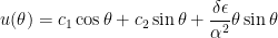
 , we find that
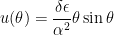
 term is what predicts the precession of a planet’s orbit under general relativity.
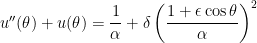 ,
,
 .
. . Since
  . Since
  , we can substitute:

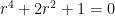
 . Factoring, we obtain
  , so that the three roots are
  and
and  . Therefore, the general solution of this differential equation is
 .
. and
and  are determined by the initial conditions. To find
 .
. .
.
 .
. .
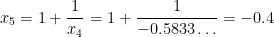
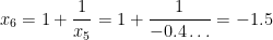
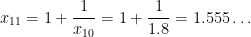
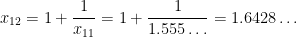
. using the quadratic formula; more on that later.) To apply the method of successive approximation, we will rewrite this so that
  , or
, or .
. .
. .
. .
. . Then
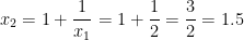
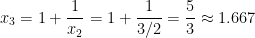
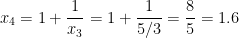


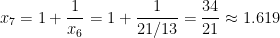
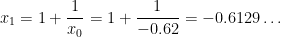
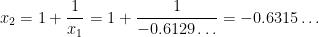
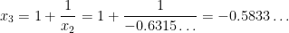
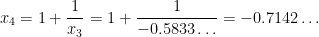
 into a calculator, then entering
  , and then repeatedly hitting the
  button.
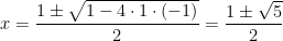 .
. .
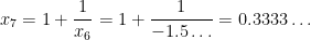
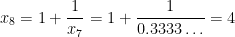
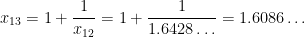
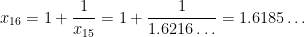
. . Unfortunately, if we start with a guess near this root, like
  , the sequence unexpectedly diverges from
  but eventually converges to the positive root
  :
:


 .
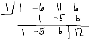
. (the constant term), while the denominator must be a factor of
  (the leading coefficient). So, using the rational root test, we conclude
 .
. and a constant
  so that
  .
.
 or
or  , I’ll tell my students: