In this series, I’m discussing how ideas from calculus and precalculus (with a touch of differential equations) can predict the precession in Mercury’s orbit and thus confirm Einstein’s theory of general relativity. The origins of this series came from a class project that I assigned to my Differential Equations students maybe 20 years ago.
But what is precession? To explore this concept, let’s explore the graph of
for various values of , , and using Desmos. (Note that, in this context, the number does not mean Euler’s constant . The reason for choosing the letter for this parameter will become clear shortly.) Naturally, this demonstration could also be done with other tools like a graphing calculator.
I suggest beginning by setting and and altering the value of . This is the easiest behavior to explain. From the equation, is directly proportional to the distance from the origin . So, not surprisingly, increasing produces a larger graph, and decreasing produces a smaller graph.
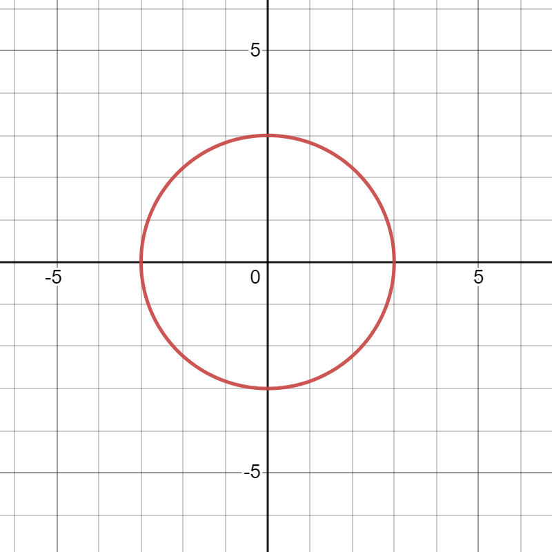
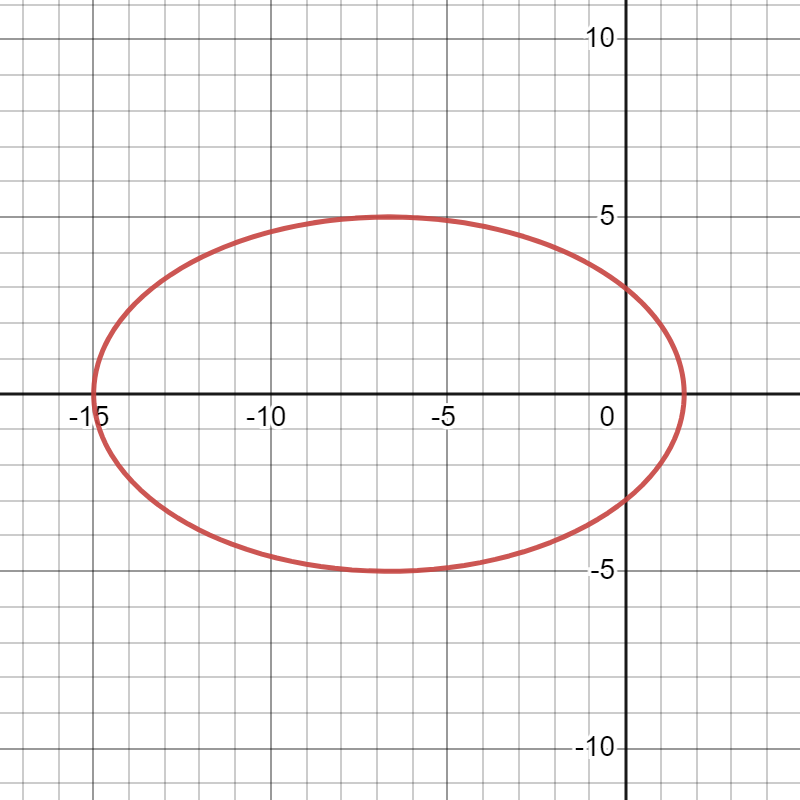
Second, I suggest setting and but altering the value of . Starting at , the graph is a circle. This makes complete sense: if , then the equation simply becomes , so the distance from the origin is the same for all angles. However, as increases, the original circle becomes more and more stretched out. We will prove this analytically in a later post, but it turns out that, for , the graph is an ellipse, and the origin is one of the foci of the ellipse. The number is called the eccentricity of the ellipse (hence the letter ).
Again, if the value of is fixed but varies, the graph becomes either larger or smaller as becomes larger or smaller.
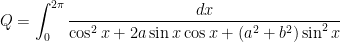
We notice that if and , then the denominator of
varies between and . In particular, the denominator is always positive. Therefore, the value of is least positive — the graph is closest to the origin — when the denominator is greatest. This happens when is a multiple of . So, for example, when , then is as close as the graph gets to the origin. Let’s call this closest distance ; in the context of a planet’s orbit around the sun, this represent perihelion. Then we have .
When , the graph switches from an ellipse to a parabola, where the origin is the focus of the parabola. For , the graph becomes a hyperbola. However, since we’re mostly going to be concerned with stable planetary orbits in this series, we won’t dwell too much on the case .
Third, I suggest setting , , and then alter the value of . For , the graph is simply a single ellipse. However, by changing the value of , the graph changes into a spiral.
In the above figure, the spiral stopped “spiraling” because I had asked Desmos only to show the graph between . If I had changed the upper bound to something larger than , the spiral would continue.
The precession in the spiral is defined to be the angular offset between each loop of the spiral. Clearly, this is a function of . To find this function, we again examine the function
Once again, if , then the denominator varies between and . In particular, the denominator is always positive. Therefore, the value of is least positive when the denominator is greatest, and the denominator is greatest when is a multiple of . So, for example, when , then is as close as the graph gets to the origin.
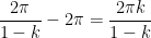
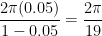
When does the graph return to its closest point to the origin next? This would occur when , or . If , then the angle of closest approach to the origin would , and the graph simply cycles over itself. However, if , then this angle will be larger than , thus producing a spiral. Indeed, the amount of precession would be equal to
.
In the picture above, . Therefore, the amount of precession would be radians . Therefore, after 19 “leafs” of the spiral, the graph would begin to cycle on top of itself.
In this series, I’m discussing how ideas from calculus and precalculus (with a touch of differential equations) can predict the precession in Mercury’s orbit and thus confirm Einstein’s theory of general relativity. The origins of this series came from a class project that I assigned to my Differential Equations students maybe 20 years ago.
This is going to be a very long series, so I’d like to provide a tree-top view of how the argument will unfold.
We begin by using three principles from Newtonian physics — the Law of Conservation of Angular Momentum, Newton’s Second Law, and Newton’s Law of Gravitation — to show that the orbit of a planet, under Newtonian physics, satisfies the initial-value problem
,
,
.
In these equations:
The orbit of the planet is in polar coordinates , where the Sun is placed at the origin.
The planet’s perihelion — closest distance from the Sun — is a distance of at angle .
The function is equal to .
is the gravitational constant of the universe.
is the mass of the Sun.
is the mass of the planet.
is the angular momentum of the planet.
The solution of this differential equation is
,
so that
.
In polar coordinates, this is the graph of an ellipse. Substituting , we see that
.
In the solution for , we have and . The number is the eccentricity of the ellipse, while is proportional to the size of the ellipse.
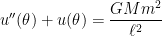
Under general relativity, the governing initial-value problem changes to
,
,
,
where is the speed of light. We will see that the solution of this new differential equation can be well approximated by
.
This last equation describes a spiral that precesses by approximately
radians per orbit
or
radians per orbit,
where is the length of the semimajor axis of the orbit.
This matches the amount of precession in Mercury’s orbit that is not explained by Newtonian physics, thus confirming Einstein’s theory of general relativity.
To the extent possible, I will take the perspective of a good student who has taken Precalculus and Calculus I. However, I will have to break this perspective a couple of times when I discuss principles from physics and derive the solutions of the above differential equations.
In this series, I’m discussing how ideas from calculus and precalculus (with a touch of differential equations) can predict the precession in Mercury’s orbit and thus confirm Einstein’s theory of general relativity. The origins of this series came from a class project that I assigned to my Differential Equations students maybe 20 years ago.
The figure below shows the (greatly exaggerated) effect of precession on a planet’s otherwise elliptical orbit. In the figure, each perihelion is precessed by an angle of . After nine orbits, the planet returns to its original position. Suppose, for the sake of argument, that each orbit of the planet depicted in the figure is four months, or one third of Earth’s year. Then the amount of precession would be per four months, or per year, or per century.
As I said, the figure above is greatly exaggerated. As we’ll see by the end of this series, Einstein’s general relativity predicts that, on top of the gravitational influences of the other planets, the orbit of Mercury should precess by 43″ of arc per century. That’s a really small angle, since 1 is equal to 60′ (minutes) of arc and each 1′ is equal to 60″ (seconds) of arc, that means 1″ of arc is the same as , so that 43″ of arc per century is about per century. That’s about a million times smaller than the precession of the fictitious planet in the above figure.
How small is , really?
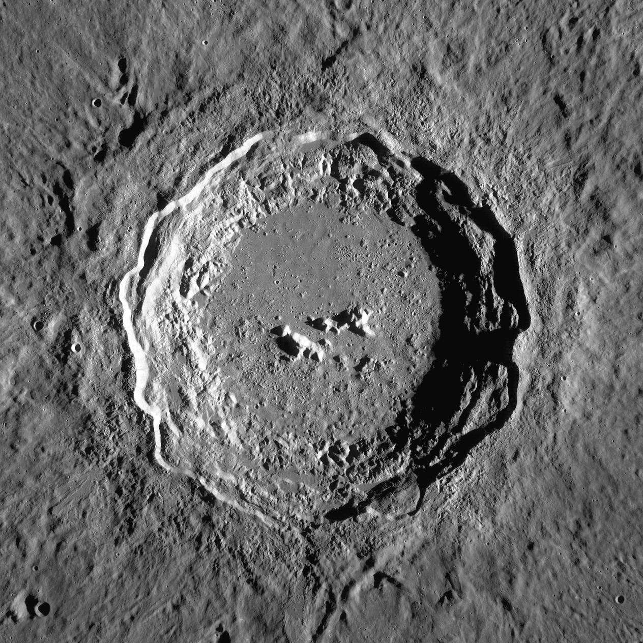
Courtesy of Wikipedia, the pictures below are the Copernicus crater on the Moon as well as an indicator of its location on the Moon. It is visible with binoculars.
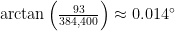
The diameter of the crater is 93 km. Since the Moon is 384,400 km from Earth, that means the angle subtended by the crater, as viewed from the Earth, is about
.
So how much is 43″ of arc per century? That’s about the speed as, hypothetically, pointing at the left edge of this lunar crater (which cannot be seen by the naked eye) and then slowly moving your figure so that, about 115 years later, your finger is pointing at the right edge of the crater.
Said another way, the diameter of the Moon is about 3475 km, so that the angle subtended by the Moon, as viewed from the Earth, is about
.
So, at the rate of per century, it would take centuries, or about 43,000 years, to trace the angle subtended by the moon.
Needless to say, 43” of arc per century is really, really slow.
Nevertheless, and remarkably, this itty, bitty precession was observable by careful 19th century astronomers with the telescopes that were available then. At the time, this precession was the great unsolved mystery of Newtonian physics that was only answered after two generations later with the discovery of general relativity.
If the universe consisted of only Mercury and the sun, Mercury’s trajectory would trace the same ellipse over and over again. However, there are seven other planets in the solar system (not to mention the dwarf planets), and these planets tug and nudge the orbit of Mercury ever so slightly. (For what it’s worth, similar nudges in the orbit of Uranus led to the discovery of Neptune in 1846.)
The practical effect of these nudges is that the orbit of Mercury precesses, or rotates like a spiral. The figure below shows the (greatly exaggerated) effect of precession on a planet’s otherwise elliptical orbit. In the figure, each perihelion is precessed by an angle of . After nine orbits, the planet returns to its original position.
Since the planets are much smaller than the sun and are further away from the Sun than Mercury, this precession is very small. However, this effect can be measured. Every century, the perihelion of Mercury precesses by 574” of arc (roughly a sixth of a degree).
Newton’s Law of Gravitation can be used to calculate the amount of the precession of Mercury; however, they predict a precession of only 531” of arc per century. This discrepancy between observation and prediction was first observed in 1845 and was, for a long time, the outstanding unresolved difficulty in Newtonian physics.
Einstein’s general theory of relativity, which was published seventy years later in 1915, exactly accounts for the missing 43” per century (within the tolerances of observational error). This was the first physical confirmation of general relativity. Furthermore, general relativity predicted that the orbit of Venus also precesses, but by only about 9” of arc per century. This small discrepancy was unobservable in 1915 but was confirmed in 1960. (While not logically necessary, that’s certainly indicative of an accurate scientific theory… not that it merely explains the world but it makes a prediction that is currently unobservable.)
In this series, which might take me a few months to complete, I’m going to explore how to predict the precession in Mercury’s orbit — i.e., confirm Einstein’s theory of general relativity — using tools only from calculus and precalculus. I first introduced these ideas as a class project for my Differential Equations students maybe 20 years ago. As we’ll see, in a couple spots, ideas from first-semester differential equations can make the steps more rigorous. However, pretty much this whole series should be accessible to a good calculus student.
I should say at the outset that none of the mathematics in this series is particularly original with me. I gladly acknowledge that I first learned the ideas in this series as an undergraduate, when I took an upper-level physics course in mechanics. In particular, pretty much all of the ideas in this series can be found in the textbook Classical Dynamics of Particles and Systems, by S. T. Thornton and J. B. Marion (Brooks Cole, New York, 2003). If I’ve made any contribution, it’s the scaffolding of these ideas to make them accessible to students who won’t be taking (or haven’t yet taken) physics courses beyond the traditional first-year sequence.
In this series, I’m compiling some of the quips and one-liners that I’ll use with my students to hopefully make my lessons more memorable for them.
Here are a couple of similar problems that arise in Precalculus:
Convert the point from Cartesian coordinates into polar coordinates.
Convert the complex number into trigonometric form.
For both problems, a point is identified that is 5 steps to the right of the origin and then 5 steps below the axis (or real axis). To make this more kinesthetic, I’ll actually walk 5 paces in front of the classroom, turn right face, and then walk 5 more paces to end up at the point.
I then ask my class, “Is there a faster way to get to this point?” Naturally, they answer: Just walk straight to the point. After some work with the trigonometry, we’ll establish that
in Cartesian coordinates is equivalent to in polar coordinates, or
$5-5i$ can be rewritten as in trigonometric form.
Once this is obtained, I’ll walk it out: I’ll start at the origin, turn clockwise by 45 degrees, and then take steps to end up at the same point as before.
Continuing the lesson, I’ll ask if the numbers and , or if some other angle and/or distance could have been chosen. Someone will usually suggest a different angle, like or . I’ll demonstrate these by turning 315 degrees counterclockwise and walking 7 steps and then turning 675 degrees and walking 7 steps (getting myself somewhat dizzy in the process).
Finally, I’ll suggest turning only 135 degrees clockwise and then taking 7 steps backwards. Naturally, when I do this, I’ll do a poor man’s version of the moonwalk:
For more information, please see my series on complex numbers.
In my capstone class for future secondary math teachers, I ask my students to come up with ideas for engaging their students with different topics in the secondary mathematics curriculum. In other words, the point of the assignment was not to devise a full-blown lesson plan on this topic. Instead, I asked my students to think about three different ways of getting their students interested in the topic in the first place.
I plan to share some of the best of these ideas on this blog (after asking my students’ permission, of course).
This student submission comes from my former student Perla Perez. Her topic, from Precalculus: graphing with polar coordinates.
How does this topic extend what your students should have learned in previous courses?
Graphing polar coordinates is usually taught in a Pre-Calculus class. Students have learned about the Cartesian Coordinates and extend their knowledge to polar coordinates. Unlike Cartesian Coordinates, which represent how to get from a specific point to the point of origin (or vice versa), the polar coordinate tells us the direction by the angle, and the distance from that point to the origin. Students will need to know how to take the measure of an angle and how to use the Pythagorean Theorem to solve for the distance which is considered the radius. Most students who are enrolled in a Pre-Calculus class have taken geometry where they have learned about the Pythagorean Theorem and what a radius is. This alongside their algebra 1 and geometry classes means they also know how to graph and plot points.
How could you as a teacher create an activity or project that involves your topic?
Polar coordinates use a different type of graph, rather than just an x and y coordinates plane. The polar coordinate plane includes symmetrical circles surrounding the center and is given a radius creating a graph that looks like a dart board. At this point students should know what a polar coordinate is. The next step is actually graphing it.
As an activity to get students excited for the wonderful world of polar coordinates, I have created a dart board game. Using an appropriate dart board, such as a magnetic one, have the students create groups of three to four student each. The point of the game is to have students create polar coordinates. The board must be properly labeled with the angles. There will be four rounds, depending on the number of members in a group. When a member throws a dart at the board it must land on a point. Wherever it lands the students must figure out the radius and the angle of the dart to the origin. This game enables students to practice finding the radius and the angle of the dart with only their previous knowledge, labels, and each other.
What interesting things can you say about the people who contributed to the discovery and/or the development of this topic?
Throughout centuries and in all parts of the world, mathematicians and astronomers have come to shape our understanding of the polar coordinate system. Two Greek astronomers Hipparchus and Archimedes used polar coordinates in much of their work. Though they didn’t commit to the full coordinate plane, Hipparchus first begins by writing a table of chords where he was able to define stellar positions. Archimedes focused on a lot on spirals and developed what now known as the Archimedes spiral, in which the radius depends on the angle. Descartes also used a simpler concept of coordinates, but relating more to the x-axis. In 1671, Sir Isaac Newton was one of the biggest contributors to the elements used in analytic geometry. The idea of polar coordinates, however, comes from a man named Gregorio Fontana (1735-1803), centuries later. Astronomers now use his polar coordinates to measure the distance of the sky and stars.
Earlier in this series, I gave three different methods of showing that
Using the fact that is independent of , I’ll now give a fourth method. Since is independent of , I can substitute any convenient value of that I want without changing the value of . As shown in previous posts, substituting yields the following simplification:
The four roots of the denominator satisfy
So far, I’ve handled the cases and . In today’s post, I’ll start considering the case .
Factoring the denominator is a bit more complicated if . Using the quadratic equation, we obtain
However, unlike the cases , the right-hand side is now a complex number. So, To solve for , I’ll use DeMoivre’s Theorem and some surprisingly convenient trig identities. Notice that
.
Therefore, the four complex roots of the denominator satisfy , or . This means that all four roots can be written in trigonometric form so that
,
where is some angle. (I chose the angle to be instead of for reasons that will become clear shortly.)
I’ll begin with solving
.
Matching the real and imaginary parts, we see that
,
This completely matches the form of the double-angle trig identities
,
,
and so the problem reduces to solving
,
where $\sin \phi = |b|$ and $\cos \phi = \sqrt{1-b^2}$. By De Moivre’s Theorem, I can conclude that the two solutions of this equation are
,
or
.
I could re-run this argument to solve and get the other two complex roots. However, by the Conjugate Root Theorem, I know that the four complex roots of the denominator must come in conjugate pairs. Therefore, the four complex roots are
.
Therefore, I can factor the denominator as follows:
To double-check my work, I can directly multiply this product:
.
So, at last, I can rewrite the integral as
I’ll continue with this fourth evaluation of the integral, continuing the case , in tomorrow’s post.
In my capstone class for future secondary math teachers, I ask my students to come up with ideas for engaging their students with different topics in the secondary mathematics curriculum. In other words, the point of the assignment was not to devise a full-blown lesson plan on this topic. Instead, I asked my students to think about three different ways of getting their students interested in the topic in the first place.
I plan to share some of the best of these ideas on this blog (after asking my students’ permission, of course).
This student submission comes from my former student Laura Lozano. Her topic, from Precalculus: graphing with polar coordinates.
How could you as a teacher create an activity or project that involves your topic?
An activity that I believe will go really well with graphing polar coordinates or any type of graphing lesson will be to convert the classroom floor into a graph. Also, I will have a selection of random objects like, a rubber ducky, boat, toy, etc. The size of the graph will depend on the size of classroom of course. If the classroom is really small then I would have to take this activity outdoors or maybe even the gym or anywhere with enough room for the graph and my students. The graph doesn’t have to be super big but I would use a graph no smaller than 8 feet by 8 feet area. I could create the graph lines with tape on the floor or draw them on big paper and tape the paper on the floor. I would start the activity with first talking about points on a Cartesian graph. An example could be to first have a students plot a couple points like (5, 4), (3, 6), or (-4, 2) on the board. Then transition them from Cartesian to polar coordinates by using the floor graph and have them discover how they relate by using the x and y coordinates to find the radius and the angle. Then later, after they get the hang of it, I would have the class split up into groups of two and let them choose an object, like a rubber ducky, boat, or toy, to set on the graph and have them write and tell me the point of their object.
We see radars in the news almost all the time. One category that it is usually used in is weather. The weather center uses their radars to detect for any water particles, debris, and basically anything that is in the air that could be approaching. The way that they tell if a storm or any other weather change is coming is by the radar’s omitting radio waves. The radar omits waves that then come back to the radar if the waves clash with anything in the air. The radar can detect how far an object is by the time it takes for the wave to come back. It works just like an echo! Also, recently with the search of the Malaysian airplane, we saw it used more. The news will show a clip of aircraft radar or ship radar searching for something in the air or in the ocean. Radars look almost exactly like a polar graph does. On the left is a regular polar graph. On the right is a ship’s radar. Both graphs have angles with circles.
How can technology (YouTube, Khan Academy [khanacademy.org], Vi Hart, Geometers Sketchpad, graphing calculators, etc.) be used to effectively engage students with this topic? Note: It’s not enough to say “such-and-such is a great website”; you need to explain in some detail why it’s a great website.
Graphing calculators can be used to discover polar coordinates and polar equations. I would first tell them to take out their calculators and just type in a random number from -10 to 10. I choose this interval because the graphing calculators have this window preset for graphing. I number that I randomly chose was the number 4. So I would go to the “Y=” button and type in 4. Then I would hit “GRAPH” and I should get a straight line horizontal line going through the y-axis at 4. I would then change the calculator mode and change from “FUNC” to “POL”. Then I would tell them to do the exact thing again with whatever number they chose. Once the hit “GRAPH” a circle should then come up. They then see how different polar graphs are from Cartesian graphs. Now, the graphs on a polar coordinate graph will all be circular instead of lines and curved lines like on the Cartesian graph.
Ordinarily, there are no great difficulties with logarithms as we’ve seen with the inverse trigonometric functions. That’s because the graph of satisfies the horizontal line test for any or . For example,
,
and we don’t have to worry about “other” solutions.
However, this goes out the window if we consider logarithms with complex numbers. Recall that the trigonometric form of a complex number is
where and , with in the appropriate quadrant. This is analogous to converting from rectangular coordinates to polar coordinates.
Over the past few posts, we developed the following theorem for computing in the case that is a complex number.
Definition. Let be a complex number so that . Then we define
.
Of course, this looks like what the definition ought to be if one formally applies the Laws of Logarithms to . However, this complex logarithm doesn’t always work the way you’d think it work. For example,
.
This is analogous to another situation when an inverse function is defined using a restricted domain, like
or
.
The Laws of Logarithms also may not work when nonpositive numbers are used. For example,


 ,
, ,
, .
. , where the Sun is placed at the origin.
 is equal to
  .
. is the gravitational constant of the universe.
 is the mass of the Sun.
 is the mass of the planet.
 is the angular momentum of the planet.
 ,
, .
. .
. and
and  . The number
  is the eccentricity of the ellipse, while
  is proportional to the size of the ellipse.
![u''(\theta) + u(\theta) = \displaystyle \frac{GMm^2}{\ell^2} + \frac{3GM}{c^2} [u(\theta)]^2](https://s0.wp.com/latex.php?latex=u%27%27%28%5Ctheta%29+%2B+u%28%5Ctheta%29+%3D+%5Cdisplaystyle+%5Cfrac%7BGMm%5E2%7D%7B%5Cell%5E2%7D+%2B+%5Cfrac%7B3GM%7D%7Bc%5E2%7D+%5Bu%28%5Ctheta%29%5D%5E2&bg=ffffff&fg=000000&s=0&c=20201002) ,
, is the speed of light. We will see that the solution of this new differential equation can be well approximated by
![\approx \displaystyle \frac{1}{\alpha} \left[1 + \epsilon \cos \left(\theta - \frac{\delta \theta}{\alpha} \right) \right]](https://s0.wp.com/latex.php?latex=%5Capprox+%5Cdisplaystyle+%5Cfrac%7B1%7D%7B%5Calpha%7D+%5Cleft%5B1+%2B+%5Cepsilon+%5Ccos+%5Cleft%28%5Ctheta+-+%5Cfrac%7B%5Cdelta+%5Ctheta%7D%7B%5Calpha%7D+%5Cright%29+%5Cright%5D&bg=ffffff&fg=000000&s=0&c=20201002) .
. radians per orbit
 radians per orbit,
 . After nine orbits, the planet returns to its original position. Suppose, for the sake of argument, that each orbit of the planet depicted in the figure is four months, or one third of Earth’s year. Then the amount of precession would be
  per four months, or
  per year, or
  per century.
 is equal to 60′ (minutes) of arc and each 1′ is equal to 60″ (seconds) of arc, that means 1″ of arc is the same as
  , so that 43″ of arc per century is about
  per century. That’s about a million times smaller than the precession of the fictitious planet in the above figure.
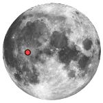
 .
. .
. centuries, or about 43,000 years, to trace the angle subtended by the moon.
  from Cartesian coordinates into polar coordinates.
 into trigonometric form.
 axis (or real axis). To make this more kinesthetic, I’ll actually walk 5 paces in front of the classroom, turn right face, and then walk 5 more paces to end up at the point.
 in polar coordinates, or
![5\sqrt{2} [ \cos(-\pi/4) + i \sin (-\pi/4)]](https://s0.wp.com/latex.php?latex=5%5Csqrt%7B2%7D+%5B+%5Ccos%28-%5Cpi%2F4%29+%2B+i+%5Csin+%28-%5Cpi%2F4%29%5D&bg=ffffff&fg=000000&s=0&c=20201002) in trigonometric form.
in trigonometric form. steps to end up at the same point as before.
 and
and  , or if some other angle and/or distance could have been chosen. Someone will usually suggest a different angle, like
  or
or  . I’ll demonstrate these by turning 315 degrees counterclockwise and walking 7 steps and then turning 675 degrees and walking 7 steps (getting myself somewhat dizzy in the process).
 is independent of
  yields the following simplification:


 and
and  . In today’s post, I’ll start considering the case
  .
.
 , the right-hand side is now a complex number. So, To solve for
  , I’ll use
  .
. , or
, or  . This means that all four roots can be written in
  ,
, is some angle. (I chose the angle to be
  for reasons that will become clear shortly.)
 .
. ,
,
 ,
, ,
, ,
, .
. and get the other two complex roots. However, by the Conjugate Root Theorem, I know that the four complex roots of the denominator
  must come in conjugate pairs. Therefore, the four complex roots are
 .
.![u^4 + (4 b^2 - 2) u^2 + 1 = (u - [\sqrt{1-b^2} + i|b|])(u - [\sqrt{1-b^2} - i|b|])](https://s0.wp.com/latex.php?latex=u%5E4+%2B+%284+b%5E2+-+2%29+u%5E2+%2B+1+%3D+%28u+-+%5B%5Csqrt%7B1-b%5E2%7D+%2B+i%7Cb%7C%5D%29%28u+-+%5B%5Csqrt%7B1-b%5E2%7D+-+i%7Cb%7C%5D%29&bg=ffffff&fg=000000&s=0&c=20201002)
![\qquad \times (u - [-\sqrt{1-b^2} + i|b|])(u - [-\sqrt{1-b^2} + i|b|])](https://s0.wp.com/latex.php?latex=%5Cqquad+%5Ctimes+%28u+-+%5B-%5Csqrt%7B1-b%5E2%7D+%2B+i%7Cb%7C%5D%29%28u+-+%5B-%5Csqrt%7B1-b%5E2%7D+%2B+i%7Cb%7C%5D%29&bg=ffffff&fg=000000&s=0&c=20201002)
![= (u - \sqrt{1-b^2} - i|b|)(u - \sqrt{1-b^2} + i|b])](https://s0.wp.com/latex.php?latex=%3D+%28u+-+%5Csqrt%7B1-b%5E2%7D+-+i%7Cb%7C%29%28u+-+%5Csqrt%7B1-b%5E2%7D+%2B+i%7Cb%5D%29&bg=ffffff&fg=000000&s=0&c=20201002)

![= ([u - \sqrt{1-b^2}]^2 +b^2)([u + \sqrt{1-b^2}]^2 +b^2)](https://s0.wp.com/latex.php?latex=%3D+%28%5Bu+-+%5Csqrt%7B1-b%5E2%7D%5D%5E2+%2Bb%5E2%29%28%5Bu+%2B+%5Csqrt%7B1-b%5E2%7D%5D%5E2+%2Bb%5E2%29&bg=ffffff&fg=000000&s=0&c=20201002)
![([u - \sqrt{1-b^2}]^2 +b^2)([u + \sqrt{1-b^2}]^2 +b^2)](https://s0.wp.com/latex.php?latex=%28%5Bu+-+%5Csqrt%7B1-b%5E2%7D%5D%5E2+%2Bb%5E2%29%28%5Bu+%2B+%5Csqrt%7B1-b%5E2%7D%5D%5E2+%2Bb%5E2%29&bg=ffffff&fg=000000&s=0&c=20201002)

![= ([u^2 +1] - 2u\sqrt{1-b^2})([u^2+1] + 2u\sqrt{1-b^2})](https://s0.wp.com/latex.php?latex=%3D+%28%5Bu%5E2+%2B1%5D+-+2u%5Csqrt%7B1-b%5E2%7D%29%28%5Bu%5E2%2B1%5D+%2B+2u%5Csqrt%7B1-b%5E2%7D%29&bg=ffffff&fg=000000&s=0&c=20201002)
![= [u^2+1]^2 - [2u\sqrt{1-b^2}]^2](https://s0.wp.com/latex.php?latex=%3D+%5Bu%5E2%2B1%5D%5E2+-+%5B2u%5Csqrt%7B1-b%5E2%7D%5D%5E2&bg=ffffff&fg=000000&s=0&c=20201002)

![= u^4 + u^2 (2 - 4[1-b^2]) + 1](https://s0.wp.com/latex.php?latex=%3D+u%5E4+%2B+u%5E2+%282+-+4%5B1-b%5E2%5D%29+%2B+1&bg=ffffff&fg=000000&s=0&c=20201002)
 .
.![Q = \displaystyle \int_{-\infty}^{\infty} \frac{ 2(1+u^2) du}{ ([u - \sqrt{1-b^2}]^2 +b^2)([u + \sqrt{1-b^2}]^2 +b^2)}](https://s0.wp.com/latex.php?latex=Q+%3D+%5Cdisplaystyle+%5Cint_%7B-%5Cinfty%7D%5E%7B%5Cinfty%7D+%5Cfrac%7B+2%281%2Bu%5E2%29+du%7D%7B+%28%5Bu+-+%5Csqrt%7B1-b%5E2%7D%5D%5E2+%2Bb%5E2%29%28%5Bu+%2B+%5Csqrt%7B1-b%5E2%7D%5D%5E2+%2Bb%5E2%29%7D&bg=ffffff&fg=000000&s=0&c=20201002)


 satisfies the horizontal line test for any
  or
or  . For example,
 ,
, is
is
 and
and  , with
  in the case that
  is a complex number.
 be a complex number so that
  . Then we define
 .
. . However, this complex logarithm doesn’t always work the way you’d think it work. For example,
 .
.
 .
.![\log \left[ (-1) \cdot (-1) \right] = \log 1 = 0](https://s0.wp.com/latex.php?latex=%5Clog+%5Cleft%5B+%28-1%29+%5Ccdot+%28-1%29+%5Cright%5D+%3D+%5Clog+1+%3D+0&bg=ffffff&fg=000000&s=0&c=20201002) ,
, .
.