Solving Problems Submitted to MAA Journals (Part 6e)

The following problem appeared in Volume 97, Issue 3 (2024) of Mathematics Magazine.

Two points $P$ and $Q$ are chosen at random (uniformly) from the interior of a unit circle. What is the probability that the circle whose diameter is segment $overline{PQ}$ lies entirely in the interior of the unit circle?

Let $D_r$ be the interior of the circle centered at the origin $O$ with radius $r$ . Also, let $C(P,Q)$ denote the circle with diameter $\overline{PQ}$ , and let $R = OP$ be the distance of $P$ from the origin.

In the previous post, we showed that

$\hbox{Pr}(C(P,Q) \subset D_1 \mid R = r) = \sqrt{1-r^2}$ .

To find $\hbox{Pr}(C(P,Q) \subset D_1)$ , I will integrate over this conditional probability:

$\hbox{Pr}(C(P,Q) \subset D_1) = \displaystyle \int_0^1 \hbox{Pr}(C(P,Q) \subset D_1 \mid R = r) F'(r) \, dr$ ,

where $F(r)$ is the cumulative distribution function of $R$ . For $0 \le r \le 1$ ,

$F(r) = \hbox{Pr}(R \le r) = \hbox{Pr}(P \in D_r) = \displaystyle \frac{\hbox{area}(D_r)}{\hbox{area}(D_1)} = \frac{\pi r^2}{\pi} = r^2$ .

Therefore,

$\hbox{Pr}(C(P,Q) \subset D_1) = \displaystyle \int_0^1 \hbox{Pr}(C(P,Q) \subset D_1 \mid R = r) F'(r) \, dr$

$= \displaystyle \int_0^1 2 r \sqrt{1-r^2} \, dr$ .

To calculate this integral, I’ll use the trigonometric substitution $u = 1-r^2$ . Then the endpoints $r=0$ and $r=1$ become $u = \sqrt{1-0^2} = 1$ and $u = \sqrt{1-1^2} = 0$ . Also, $du = -2r \, dr$ . Therefore,

$\hbox{Pr}(C(P,Q) \subset D_1) = \displaystyle \int_0^1 2 r \sqrt{1-r^2} \, dr$

$= \displaystyle \int_1^0 -\sqrt{u} \, du$

$= \displaystyle \int_0^1 \sqrt{u} \, du$

$= \displaystyle \frac{2}{3} \left[ u^{3/2} \right]_0^1$

$=\displaystyle \frac{2}{3}\left[ (1)^{3/2} - (0)^{3/2} \right]$

$= \displaystyle \frac{2}{3}$ ,

confirming the answer I had guessed from simulations.

Confirming Einstein’s Theory of General Relativity With Calculus, Part 5d: Deriving Orbits under Newtonian Mechanics Using Variation of Parameters

In this series, I’m discussing how ideas from calculus and precalculus (with a touch of differential equations) can predict the precession in Mercury’s orbit and thus confirm Einstein’s theory of general relativity. The origins of this series came from a class project that I assigned to my Differential Equations students maybe 20 years ago.

We previously showed that if the motion of a planet around the Sun is expressed in polar coordinates $(r,theta)$ , with the Sun at the origin, then under Newtonian mechanics (i.e., without general relativity) the motion of the planet follows the differential equation

$u''(\theta) + u(\theta) = \displaystyle \frac{1}{\alpha}$ ,

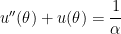
where $u = 1/r$ and $\alpha$ is a certain constant. We will also impose the initial condition that the planet is at perihelion (i.e., is closest to the sun), at a distance of $P$ , when $\theta = 0$ . This means that $u$ obtains its maximum value of $1/P$ when $\theta = 0$ . This leads to the two initial conditions

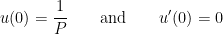$u(0) = \displaystyle \frac{1}{P} \qquad \hbox{and} \qquad u'(0) = 0$ ;

the second equation arises since $u$ has a local extremum at $\theta = 0$ .

We now take the perspective of a student who is taking a first-semester course in differential equations. There are two standard techniques for solving a second-order non-homogeneous differential equations with constant coefficients. One of these is the method of variation of parameters. First, we solve the associated homogeneous differential equation

$u''(\theta) + u(\theta) = 0$ .

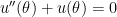The characteristic equation of this differential equation is $r^2 + 1 = 0$ , which clearly has the two imaginary roots $r = \pm i$ . Therefore, two linearly independent solutions of the associated homogeneous equation are $u_1(\theta) = \cos \theta$ and $u_2(\theta) = \sin \theta$ .

(As an aside, this is one answer to the common question, “What are complex numbers good for?” The answer is naturally above the heads of Algebra II students when they first encounter the mysterious number $i$ , but complex numbers provide a way of solving the differential equations that model multiple problems in statics and dynamics.)

According to the method of variation of parameters, the general solution of the original nonhomogeneous differential equation

$u''(\theta) + u(\theta) = g(\theta)$

$u(\theta) = f_1(\theta) u_1(\theta) + f_2(\theta) u_2(\theta)$ ,

where

$f_1(\theta) = -\displaystyle \int \frac{u_2(\theta) g(\theta)}{W(\theta)} d\theta$ ,

$f_2(\theta) = \displaystyle \int \frac{u_1(\theta) g(\theta)}{W(\theta)} d\theta$ ,

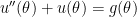
and $W(\theta)$ is the Wronskian of $u_1(\theta)$ and $u_2(\theta)$ , defined by the determinant

$W(\theta) = \displaystyle \begin{vmatrix} u_1(\theta) & u_2(\theta) \\ u_1'(\theta) & u_2'(\theta) \end{vmatrix} = u_1(\theta) u_2'(\theta) - u_1'(\theta) u_2(\theta)$ .

Well, that’s a mouthful.

Fortunately, for the example at hand, these computations are pretty easy. First, since $u_1(\theta) = \cos \theta$ and $u_2(\theta) = \sin \theta$ , we have

$W(\theta) = (\cos \theta)(\cos \theta) - (\sin \theta)(-\sin \theta) = \cos^2 \theta + \sin^2 \theta = 1$

from the usual Pythagorean trigonometric identity. Therefore, the denominators in the integrals for $f_1(\theta)$ and $f_2(\theta)$ essentially disappear.

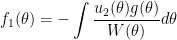
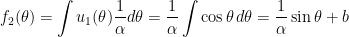
Since $g(\theta) = \displaystyle \frac{1}{\alpha}$ , the integrals for $f_1(\theta)$ and $f_2(\theta)$ are straightforward to compute:

$f_1(\theta) = -\displaystyle \int u_2(\theta) \frac{1}{\alpha} d\theta = -\displaystyle \frac{1}{\alpha} \int \sin \theta \, d\theta = \displaystyle \frac{1}{\alpha}\cos \theta + a$ ,

where we use $+a$ for the constant of integration instead of the usual $+C$ . Second,

$f_2(\theta) = \displaystyle \int u_1(\theta) \frac{1}{\alpha} d\theta = \displaystyle \frac{1}{\alpha} \int \cos \theta \, d\theta = \displaystyle \frac{1}{\alpha}\sin \theta + b$ ,

using $+b$ for the constant of integration. Therefore, by variation of parameters, the general solution of the nonhomogeneous differential equation is

$u(\theta) = f_1(\theta) u_1(\theta) + f_2(\theta) u_2(\theta)$

$= \left( \displaystyle \frac{1}{\alpha}\cos \theta + a \right) \cos \theta + \left( \displaystyle \frac{1}{\alpha}\sin\theta + b \right) \sin \theta$

$= a \cos \theta + b\sin \theta + \displaystyle \frac{\cos^2 \theta + \sin^2 \theta}{\alpha}$

$= a \cos \theta + b \sin \theta + \displaystyle \frac{1}{\alpha}$ .

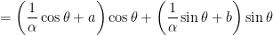
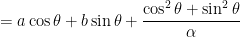
Unsurprisingly, this matches the answer in the previous post that was found by the method of undetermined coefficients.

For the sake of completeness, I repeat the argument used in the previous two posts to determine $a$ and $b$ . This is require using the initial conditions $u(0) = \displaystyle \frac{1}{P}$ and $u'(0) = 0$ . From the first initial condition,

$u(0) = a \cos 0 + b \sin 0 + \displaystyle \frac{1}{\alpha}$

$\displaystyle \frac{1}{P} = a + \frac{1}{\alpha}$

$\displaystyle \frac{1}{P} - \frac{1}{\alpha} = a$

$\displaystyle \frac{\alpha - P}{\alpha P} = a$

From the second initial condition,

$u'(\theta) = -a \sin \theta + b \cos \theta$

$u'(0) = -a \sin 0 + b \cos 0$

$0 = b$ .

From these two constants, we obtain

$u(\theta) = \displaystyle \frac{\alpha - P}{\alpha P} \cos \theta + 0 \sin \theta + \displaystyle \frac{1}{\alpha}$

$= \displaystyle \frac{1}{\alpha} \left( 1 + \frac{\alpha-P}{P} \cos \theta \right)$

$= \displaystyle \frac{1 + \epsilon \cos \theta}{\alpha}$ ,

where $\epsilon = \displaystyle \frac{\alpha - P}{P}$ .

Finally, since $r = 1/u$ , we see that the planet’s orbit satisfies

$r = \displaystyle \frac{\alpha}{1 + \epsilon \cos \theta}$ ,

so that, as shown earlier in this series, the orbit is an ellipse with eccentricity $\epsilon$ .

Thoughts on Numerical Integration (Part 23): The normalcdf function on TI calculators

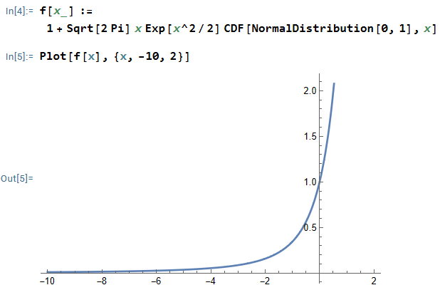
I end this series about numerical integration by returning to the most common (if hidden) application of numerical integration in the secondary mathematics curriculum: finding the area under the normal curve. This is a critically important tool for problems in both probability and statistics; however, the antiderivative of $\displaystyle \frac{1}{\sqrt{2\pi}} e^{-x^2/2}$ cannot be expressed using finitely many elementary functions. Therefore, we must resort to numerical methods instead.

In days of old, of course, students relied on tables in the back of the textbook to find areas under the bell curve, and I suppose that such tables are still being printed. For students with access to modern scientific calculators, of course, there’s no need for tables because this is a built-in function on many calculators. For the line of TI calculators, the command is normalcdf.

Unfortunately, it’s a sad (but not well-known) fact of life that the TI-83 and TI-84 calculators are not terribly accurate at computing these areas. For example:

TI-84: $\displaystyle \int_0^1 \frac{e^{-x^2/2}}{\sqrt{2\pi}} \, dx \approx 0.3413447\underline{399}$

Correct answer, with Mathematica: $0.3413447\underline{467}\dots$

TI-84: $\displaystyle \int_1^2 \frac{e^{-x^2/2}}{\sqrt{2\pi}} \, dx \approx 0.1359051\underline{975}$

Correct answer, with Mathematica: $0.1359051\underline{219}\dots$

TI-84: $\displaystyle \int_2^3 \frac{e^{-x^2/2}}{\sqrt{2\pi}} \, dx \approx 0.021400\underline{0948}$

Correct answer, with Mathematica: $0.021400\underline{2339}\dots$

TI-84: $\displaystyle \int_3^4 \frac{e^{-x^2/2}}{\sqrt{2\pi}} \, dx \approx 0.0013182\underline{812}$

Correct answer, with Mathematica: $0.0013182\underline{267}\dots$

TI-84: $\displaystyle \int_4^5 \frac{e^{-x^2/2}}{\sqrt{2\pi}} \, dx \approx 0.0000313\underline{9892959}$

Correct answer, with Mathematica: $0.0000313\underline{84590261}\dots$

TI-84: $\displaystyle \int_5^6 \frac{e^{-x^2/2}}{\sqrt{2\pi}} \, dx \approx 2.8\underline{61148776} \times 10^{-7}$

Correct answer, with Mathematica: $2.8\underline{56649842}\dots \times 10^{-7}$

I don’t presume to know the proprietary algorithm used to implement normalcdf on TI-83 and TI-84 calculators. My honest if brutal assessment is that it’s probably not worth knowing: in the best case (when the endpoints are close to 0), the calculator provides an answer that is accurate to only 7 significant digits while presenting the illusion of a higher degree of accuracy. 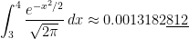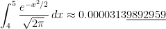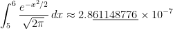I can say that Simpson’s Rule with only $n = 26$ subintervals provides a better approximation to $\displaystyle \int_0^1 \frac{e^{-x^2/2}}{\sqrt{2\pi}} \, dx$ than the normalcdf function.

For what it’s worth, I also looked at the accuracy of the NORMSDIST function in Microsoft Excel. This is much better, almost always producing answers that are accurate to 11 or 12 significant digits, which is all that can be realistically expected in floating-point double-precision arithmetic (in which numbers are usually stored accurate to 13 significant digits prior to any computations).

Thoughts on Numerical Integration (Part 22): Comparison to theorems about magnitudes of errors

Numerical integration is a standard topic in first-semester calculus. From time to time, I have received questions from students on various aspects of this topic, including:

Why is numerical integration necessary in the first place?
Where do these formulas come from (especially Simpson’s Rule)?
How can I do all of these formulas quickly?
Is there a reason why the Midpoint Rule is better than the Trapezoid Rule?
Is there a reason why both the Midpoint Rule and the Trapezoid Rule converge quadratically?
Is there a reason why Simpson’s Rule converges like the fourth power of the number of subintervals?

In this series, I hope to answer these questions. While these are standard questions in a introductory college course in numerical analysis, and full and rigorous proofs can be found on Wikipedia and Mathworld, I will approach these questions from the point of view of a bright student who is currently enrolled in calculus and hasn’t yet taken real analysis or numerical analysis.

In this series, we have shown the following approximations of errors when using various numerical approximations for $\int_a^b x^k \, dx$ . We obtained these approximations using only techniques within the reach of a talented high school student who has mastered Precalculus — especially the Binomial Theorem — and elementary techniques of integration.

As we now present, the formulas that we derived are (of course) easily connected to known theorems for the convergence of these techniques. These proofs, however, require some fairly advanced techniques from calculus. So, while the formulas derived in this series of posts only apply to $f(x) = x^k$ (and, by an easy extension, any polynomial), the formulas that we do obtain easily foreshadow the actual formulas found on Wikipedia or Mathworld or calculus textbooks, thus (hopefully) taking some of the mystery out of these formulas.

Left and right endpoints: Our formula was

$E \approx \displaystyle \frac{k}{2} x_*^{k-1} (b-a)h$ ,

where $x_*$ is some number between $a$ and $b$ . By comparison, the actual formula for the error is

$E = \displaystyle \frac{f'(x_*) (b-a)^2}{2n} = \frac{f'(x_*)}{2} (b-a)h$ .

This reduces to the formula that we derived since $f'(x) = kx^{k-1}$ .

Midpoint Rule: Our formula was

$E \approx \displaystyle \frac{k(k-1)}{24} x_*^{k-1} (b-a)h$ ,

where $x_*$ is some number between $a$ and $b$ . By comparison, the actual formula for the error is

E = \displaystyle \frac{f''(x_*) (b-a)^3}{24n^2} = \frac{f''(x_*)}{24} (b-a)h^2

This reduces to the formula that we derived since $f''(x) = k(k-1)x^{k-2}$ .

Trapezoid Rule: Our formula was

$E \approx \displaystyle \frac{k(k-1)}{12} x_*^{k-1} (b-a)h$ ,

where $x_*$ is some number between $a$ and $b$ . By comparison, the actual formula for the error is

$E = \displaystyle \frac{f''(x_*) (b-a)^3}{12n^2} = \frac{f''(x_*)}{12} (b-a)h^2$ .

This reduces to the formula that we derived since $f''(x) = k(k-1)x^{k-2}$ .

Simpson’s Rule: Our formula was

$E \approx \displaystyle \frac{k(k-1)(k-2)(k-3)}{180} x_*^{k-4} (b-a)h^4$ ,

where $x_*$ is some number between $a$ and $b$ . By comparison, the actual formula for the error is

$E = \displaystyle \frac{f^{(4)}(x_*)}{180} (b-a)h^4$ .

This reduces to the formula that we derived since $f^{(4)}(x) = k(k-1)(k-2)(k-3)x^{k-4}$ .

Thoughts on Numerical Integration (Part 21): Simpson’s rule and global rate of convergence

Numerical integration is a standard topic in first-semester calculus. From time to time, I have received questions from students on various aspects of this topic, including:

Why is numerical integration necessary in the first place?
Where do these formulas come from (especially Simpson’s Rule)?
How can I do all of these formulas quickly?
Is there a reason why the Midpoint Rule is better than the Trapezoid Rule?
Is there a reason why both the Midpoint Rule and the Trapezoid Rule converge quadratically?
Is there a reason why Simpson’s Rule converges like the fourth power of the number of subintervals?

In this previous post in this series, we showed that the Simpson’s Rule approximation of $\displaystyle \int_{x_i}^{x_i+2h} x^k \, dx$ has an error of

$-\displaystyle \frac{k(k-1)(k-2)(k-3)}{90} x_i^{k-4} h^5 + O(h^6)$ .

Thoughts on Numerical Integration (Part 20): Simpson’s rule and local rate of convergence

Numerical integration is a standard topic in first-semester calculus. From time to time, I have received questions from students on various aspects of this topic, including:

Why is numerical integration necessary in the first place?
Where do these formulas come from (especially Simpson’s Rule)?
How can I do all of these formulas quickly?
Is there a reason why the Midpoint Rule is better than the Trapezoid Rule?
Is there a reason why both the Midpoint Rule and the Trapezoid Rule converge quadratically?
Is there a reason why Simpson’s Rule converges like the fourth power of the number of subintervals?

In this post, we will perform an error analysis for Simpson’s Rule

$\int_a^b f(x) \, dx \approx \frac{h}{3} \left[f(x_0) + 4(x_1) + 2f(x_2) + \dots + 2f(x_{n-2}) + 4f(x_{n-1}) +f(x_n) \right] \equiv T_n$

where $n$ is the number of subintervals (which has to be even) and $h = (b-a)/n$ is the width of each subinterval, so that $x_k = x_0 + kh$ .

For this special case, the true area under the curve $f(x) = x^k$ on the subinterval $[x_i, x_i +h]$ will be

$\displaystyle \int_{x_i}^{x_i+h} x^k \, dx = \frac{1}{k+1} \left[ (x_i+h)^{k+1} - x_i^{k+1} \right]$

$= \displaystyle \frac{1}{k+1} \left[x_i^{k+1} + {k+1 \choose 1} x_i^k h + {k+1 \choose 2} x_i^{k-1} h^2 + {k+1 \choose 3} x_i^{k-2} h^3 + {k+1 \choose 4} x_i^{k-3} h^4+ {k+1 \choose 5} x_i^{k-4} h^5+ O(h^6) - x_i^{k+1} \right]$

$= \displaystyle \frac{1}{k+1} \bigg[ (k+1) x_i^k h + \frac{(k+1)k}{2} x_i^{k-1} h^2 + \frac{(k+1)k(k-1)}{6} x_i^{k-2} h^3+ \frac{(k+1)k(k-1)(k-2)}{24} x_i^{k-3} h^4$

$+ \displaystyle \frac{(k+1)k(k-1)(k-2)(k-3)}{120} x_i^{k-4} h^5 \bigg] + O(h^6)$

$= x_i^k h + \displaystyle \frac{k}{2} x_i^{k-1} h^2 + \frac{k(k-1)}{6} x_i^{k-2} h^3 + \frac{k(k-1)(k-2)}{24} x_i^{k-3} h^4 + \frac{k(k-1)(k-2)(k-3)}{120} x_i^{k-4} h^5 + O(h^6)$

Earlier in this series, we derived the very convenient relationship $S_{2n} = \displaystyle \frac{2}{3} M_n + \frac{1}{3} T_n$ relating the approximations from Simpson’s Rule, the Midpoint Rule, and the Trapezoid Rule. We now exploit this relationship to approximate $\displaystyle \int_{x_i}^{x_i+h} x^k \, dx$ . Earlier in this series, we found the Midpoint Rule approximation on this subinterval to be

$M = x_i^k h + \displaystyle \frac{k}{2} x_i^{k-1} h^2 + \frac{k(k-1)}{8} x_i^{k-2} h^3 + \frac{k(k-1)(k-2}{48} x_i^{k-3} h^4$

$\displaystyle + \frac{k(k-1)(k-2)(k-3)}{384} x_i^{k-4} h^5 + O(h^6)$

while we found the Trapezoid Rule approximation to be

$T = x_i^k h + \displaystyle \frac{k}{2} x_i^{k-1} h^2 + \frac{k(k-1)}{4} x_i^{k-2} h^3 + \frac{k(k-1)(k-2)}{12} x_i^{k-3} h^4$

$\displaystyle + \frac{k(k-1)(k-2)(k-3)}{48} x_i^{k-4} h^5 + O(h^6)$ .

Therefore, if there are $2n$ subintervals, the Simpson’s Rule approximation of $\displaystyle \int_{x_i}^{x_i+h} x^k \, dx$ — that is, the area under the parabola that passes through $(x_i, x_i^k)$ , $(x_i + h/2, (x_i +h/2)^k)$ , and $(x_i + h, (x_i +h)^k)$ — will be $S = \frac{2}{3}M + \frac{1}{3}T$ . Since

$\displaystyle \frac{2}{3} \frac{1}{8} + \frac{1}{3} \frac{1}{4} = \frac{1}{6}$ ,

$\displaystyle \frac{2}{3} \frac{1}{48} + \frac{1}{3} \frac{1}{12} = \frac{1}{24}$ ,

and

$\displaystyle \frac{2}{3} \frac{1}{384} + \frac{1}{3} \frac{1}{48} = \frac{5}{576}$ ,

we see that

$S = x_i^k h + \displaystyle \frac{k}{2} x_i^{k-1} h^2 + \frac{k(k-1)}{6} x_i^{k-2} h^3 + \frac{k(k-1)(k-2)}{24} x_i^{k-3} h^4$

$\displaystyle + \frac{5k(k-1)(k-2)(k-3)}{576} x_i^{k-4} h^5 + O(h^6)$ .

We notice that something wonderful just happened: the first four terms of $S$ perfectly match the first four terms of the exact value of the integral! Subtracting from the actual integral, the error in this approximation will be equal to

$\displaystyle \frac{k(k-1)(k-2)(k-3)}{120} x_i^{k-4} h^5 - \frac{5k(k-1)(k-2)(k-3)}{576} x_i^{k-4} h^5 + O(h^6)$

$= -\displaystyle \frac{k(k-1)(k-2)(k-3)}{2880} x_i^{k-4} h^5 + O(h^6)$

Before moving on, there’s one minor bookkeeping issue to deal with. We note that this is the error for $S_{2n}$ , where $2n$ subintervals are used. However, the value of $h$ in this equal arose from $T_n$ and $M_n$ , where only $n$ subintervals are used. So let’s write the error with $2n$ subintervals as

$-\displaystyle \frac{k(k-1)(k-2)(k-3)}{90} x_i^{k-4} \left( \frac{h}{2} \right)^5 + O(h^6)$ ,

where $h/2$ is the width of all of the $2n$ subintervals. By analogy, we see that the error for $n$ subintervals will be

$-\displaystyle \frac{k(k-1)(k-2)(k-3)}{90} x_i^{k-4} h^5 + O(h^6)$ .

But even after adjusting for this constant, we see that this local error behaves like $O(h^5)$ , a vast improvement over both the Midpoint Rule and the Trapezoid Rule. This illustrates a general principle of numerical analysis: given two algorithms that are $O(h^3)$ , an improved algorithm can typically be made by taking some linear combination of the two algorithms. Usually, the improvement will be to $O(h^4)$ ; however, in this example, we magically obtained an improvement to $O(h^5)$ .

Thoughts on Numerical Integration (Part 19): Trapezoid rule and global rate of convergence

Numerical integration is a standard topic in first-semester calculus. From time to time, I have received questions from students on various aspects of this topic, including:

Why is numerical integration necessary in the first place?
Where do these formulas come from (especially Simpson’s Rule)?
How can I do all of these formulas quickly?
Is there a reason why the Midpoint Rule is better than the Trapezoid Rule?
Is there a reason why both the Midpoint Rule and the Trapezoid Rule converge quadratically?
Is there a reason why Simpson’s Rule converges like the fourth power of the number of subintervals?

In the previous post, we showed that the Trapezoid Rule approximation of $\displaystyle \int_{x_i}^{x_i+h} x^k \, dx$ has error

$\displaystyle \frac{k(k-1)}{12} x_i^{k-2} h^3 + O(h^4)$

In this post, we consider the global error when integrating on the interval $[a,b]$ instead of a subinterval $[x_i,x_i+h]$ . The logic is almost a perfect copy-and-paste from the analysis used for the Midpoint Rule. The total error when approximating $\displaystyle \int_a^b x^k \, dx = \int_{x_0}^{x_n} x^k \, dx$ will be the sum of the errors for the integrals over $[x_0,x_1]$ , $[x_1,x_2]$ , through $[x_{n-1},x_n]$ . Therefore, the total error will be

$E \approx \displaystyle \frac{k(k-1)}{12} \left(x_0^{k-2} + x_1^{k-2} + \dots + x_{n-1}^{k-2} \right) h^3$ .

So that this formula doesn’t appear completely mystical, this actually matches the numerical observations that we made earlier. The figure below shows the left-endpoint approximations to $\displaystyle \int_1^2 x^9 \, dx$ for different numbers of subintervals. If we take $n = 100$ and $h = 0.01$ , then the error should be approximately equal to

$\displaystyle \frac{9 \times 8}{12} \left(1^7 + 1.01^7 + \dots + 1.99^7 \right) (0.01)^3 \approx 0.0187462$ ,

which, as expected, is close to the actual error of $102.3191246 - 102.3 \approx 0.0191246$ .

Let $y_i = x_i^{k-2}$ , so that the error becomes

$E \approx \displaystyle \frac{k(k-1)}{12} \left(y_0 + y_1 + \dots + y_{n-1} \right) h^3 + O(h^4) = \displaystyle \frac{k(k-1)}{12} \overline{y} n h^3$ ,

where $\overline{y} = (y_0 + y_1 + \dots + y_{n-1})/n$ is the average of the $y_i$ . Clearly, this average is somewhere between the smallest and the largest of the $y_i$ . Since $y = x^{k-2}$ is a continuous function, that means that there must be some value of $x_*$ between $x_0$ and $x_{k-1}$ — and therefore between $a$ and $b$ — so that $x_*^{k-2} = \overline{y}$ by the Intermediate Value Theorem. We conclude that the error can be written as

$E \approx \displaystyle \frac{k(k-1)}{12} x_*^{k-2} nh^3$ ,

Finally, since $h$ is the length of one subinterval, we see that $nh = b-a$ is the total length of the interval $[a,b]$ . Therefore,

$E \approx \displaystyle \frac{k(k-1)}{12} x_*^{k-2} (b-a)h^2 \equiv ch^2$ ,

where the constant $c$ is determined by $a$ , $b$ , and $k$ . In other words, for the special case $f(x) = x^k$ , we have established that the error from the Trapezoid Rule is approximately quadratic in $h$ — without resorting to the generalized mean-value theorem and confirming the numerical observations we made earlier.

Thoughts on Numerical Integration (Part 18): Trapezoid rule and local rate of convergence

Numerical integration is a standard topic in first-semester calculus. From time to time, I have received questions from students on various aspects of this topic, including:

Why is numerical integration necessary in the first place?
Where do these formulas come from (especially Simpson’s Rule)?
How can I do all of these formulas quickly?
Is there a reason why the Midpoint Rule is better than the Trapezoid Rule?
Is there a reason why both the Midpoint Rule and the Trapezoid Rule converge quadratically?
Is there a reason why Simpson’s Rule converges like the fourth power of the number of subintervals?

In this post, we will perform an error analysis for the Trapezoid Rule

$\int_a^b f(x) \, dx \approx \frac{h}{2} \left[f(x_0) + 2f(x_1) + 2f(x_2) + \dots + 2f(x_{n-1}) +f(x_n) \right] \equiv T_n$

where $n$ is the number of subintervals and $h = (b-a)/n$ is the width of each subinterval, so that $x_k = x_0 + kh$ .

As noted above, a true exploration of error analysis requires the generalized mean-value theorem, which perhaps a bit much for a talented high school student learning about this technique for the first time. That said, the ideas behind the proof are accessible to high school students, using only ideas from the secondary curriculum (especially the Binomial Theorem), if we restrict our attention to the special case $f(x) = x^k$ , where $k \ge 5$ is a positive integer.

For this special case, the true area under the curve $f(x) = x^k$ on the subinterval $[x_i, x_i +h]$ will be

$\displaystyle \int_{x_i}^{x_i+h} x^k \, dx = \frac{1}{k+1} \left[ (x_i+h)^{k+1} - x_i^{k+1} \right]$

$= \displaystyle \frac{1}{k+1} \bigg[ (k+1) x_i^k h + \frac{(k+1)k}{2} x_i^{k-1} h^2 + \frac{(k+1)k(k-1)}{6} x_i^{k-2} h^3+ \frac{(k+1)k(k-1)(k-2)}{24} x_i^{k-3} h^4$

$+ \displaystyle \frac{(k+1)k(k-1)(k-2)(k-3)}{120} x_i^{k-4} h^5 \bigg] + O(h^6)$

$= x_i^k h + \displaystyle \frac{k}{2} x_i^{k-1} h^2 + \frac{k(k-1)}{6} x_i^{k-2} h^3 + \frac{k(k-1)(k-2)}{24} x_i^{k-3} h^4 + \frac{k(k-1)(k-2)(k-3)}{120} x_i^{k-4} h^5 + O(h^6)$

In the above, the shorthand $O(h^6)$ can be formally defined, but here we’ll just take it to mean “terms that have a factor of $h^6$ or higher that we’re too lazy to write out.” Since $h$ is supposed to be a small number, these terms will small in magnitude and thus can be safely ignored. I wrote the above formula to include terms up to and including $h^5$ because I’ll need this later in this series of posts. For now, looking only at the Trapezoid Rule, it will suffice to write this integral as

$\displaystyle \int_{x_i}^{x_i+h} x^k \, dx =x_i^k h + \displaystyle \frac{k}{2} x_i^{k-1} h^2 + \frac{k(k-1)}{6} x_i^{k-2} h^3 + O(h^4)$ .

Using the Trapezoid Rule, we approximate $\displaystyle \int_{x_i}^{x_i+h} x^k \, dx$ as $\displaystyle \frac{h}{2} \left[x_i^k + (x_i + h)^k \right]$ , using the width $h$ and the bases $x_i^k$ and $(x_i + h)^k$ of the trapezoid. Using the Binomial Theorem, this expands as

$x_i^k h + \displaystyle {k \choose 1} x_i^{k-1} \frac{h^2}{2} + {k \choose 2} x_i^{k-2} \frac{h^3}{2} + {k \choose 3} x_i^{k-3} \frac{h^4}{2} + {k \choose 4} x_i^{k-4} \frac{h^5}{2} + O(h^6)$

$= x_i^k h + \displaystyle \frac{k}{2} x_i^{k-1} h^2 + \frac{k(k-1)}{4} x_i^{k-2} h^3 + \frac{k(k-1)(k-2)}{12} x_i^{k-3} h^4$

$\displaystyle + \frac{k(k-1)(k-2)(k-3)}{48} x_i^{k-4} h^5 + O(h^6)$

Once again, this is a little bit overkill for the present purposes, but we’ll need this formula later in this series of posts. Truncating somewhat earlier, we find that the Trapezoid Rule for this subinterval gives

$x_i^k h + \displaystyle \frac{k}{2} x_i^{k-1} h^2 + \displaystyle \frac{k(k-1)}{4} x_i^{k-2} h^3 + O(h^4)$

Subtracting from the actual integral, the error in this approximation will be equal to

$\displaystyle x_i^k h + \frac{k}{2} x_i^{k-1} h^2 + \frac{k(k-1)}{6} x_i^{k-2} h^3 - x_i^k h - \frac{k}{2} x_i^{k-1} h^2 - \frac{k(k-1)}{4} x_i^{k-2} h^3 + O(h^4)$

$= \displaystyle \frac{k(k-1)}{12} x_i^{k-2} h^3 + O(h^4)$

In other words, like the Midpoint Rule, both of the first two terms $x_i^k h$ and $\displaystyle \frac{k}{2} x_i^{k-1} h^2$ cancel perfectly, leaving us with a local error on the order of $h^3$ . We also recall, from the previous post in this series that the local error from the Midpoint Rule was $\displaystyle \frac{k(k-1)}{24} x_i^{k-2} h^3 + O(h^4)$ . In other words, while both the Midpoint Rule and Trapezoid Rule have local errors on the order of $O(h^3)$ , we expect the error in the Midpoint Rule to be about half of the error from the Trapezoid Rule.

Thoughts on Numerical Integration (Part 17): Midpoint rule and global rate of convergence

Numerical integration is a standard topic in first-semester calculus. From time to time, I have received questions from students on various aspects of this topic, including:

Why is numerical integration necessary in the first place?
Where do these formulas come from (especially Simpson’s Rule)?
How can I do all of these formulas quickly?
Is there a reason why the Midpoint Rule is better than the Trapezoid Rule?
Is there a reason why both the Midpoint Rule and the Trapezoid Rule converge quadratically?
Is there a reason why Simpson’s Rule converges like the fourth power of the number of subintervals?

In the previous post, we showed that the midpoint approximation of $\displaystyle \int_{x_i}^{x_i+h} x^k \, dx$ has error

$= \displaystyle \frac{k(k-1)}{24} x_i^{k-2} h^3 + O(h^4)$

In this post, we consider the global error when integrating on the interval $[a,b]$ instead of a subinterval $[x_i,x_i+h]$ . The logic for determining the global error is much the same as what we used earlier for the left-endpoint rule. The total error when approximating $\displaystyle \int_a^b x^k \, dx = \int_{x_0}^{x_n} x^k \, dx$ will be the sum of the errors for the integrals over $[x_0,x_1]$ , $[x_1,x_2]$ , through $[x_{n-1},x_n]$ . Therefore, the total error will be

$E \approx \displaystyle \frac{k(k-1)}{24} \left(x_0^{k-2} + x_1^{k-2} + \dots + x_{n-1}^{k-2} \right) h^3$ .

$\displaystyle \frac{9 \times 8}{24} \left(1^7 + 1.01^7 + \dots + 1.99^7 \right) (0.01)^3 \approx 0.0093731$ ,

which, as expected, is close to the actual error of $102.3 - 102.2904379 \approx 0.00956211$ .

Let $y_i = x_i^{k-2}$ , so that the error becomes

$E \approx \displaystyle \frac{k(k-1)}{24} \left(y_0 + y_1 + \dots + y_{n-1} \right) h^3 + O(h^4) = \displaystyle \frac{k(k-1)}{24} \overline{y} n h^3$ ,

$E \approx \displaystyle \frac{k(k-1)}{24} x_*^{k-2} nh^3$ ,

Finally, since $h$ is the length of one subinterval, we see that $nh = b-a$ is the total length of the interval $[a,b]$ . Therefore,

$E \approx \displaystyle \frac{k(k-1)}{24} x_*^{k-2} (b-a)h^2 \equiv ch^2$ ,

where the constant $c$ is determined by $a$ , $b$ , and $k$ . In other words, for the special case $f(x) = x^k$ , we have established that the error from the Midpoint Rule is approximately quadratic in $h$ — without resorting to the generalized mean-value theorem and confirming the numerical observations we made earlier.

Thoughts on Numerical Integration (Part 16): Midpoint rule and local rate of convergence

Numerical integration is a standard topic in first-semester calculus. From time to time, I have received questions from students on various aspects of this topic, including:

Why is numerical integration necessary in the first place?
Where do these formulas come from (especially Simpson’s Rule)?
How can I do all of these formulas quickly?
Is there a reason why the Midpoint Rule is better than the Trapezoid Rule?
Is there a reason why both the Midpoint Rule and the Trapezoid Rule converge quadratically?
Is there a reason why Simpson’s Rule converges like the fourth power of the number of subintervals?

In this post, we will perform an error analysis for the Midpoint Rule

$\int_a^b f(x) \, dx \approx h \left[f(c_1) + f(c_2) + \dots + f(c_n) \right] \equiv M_n$

where $n$ is the number of subintervals and $h = (b-a)/n$ is the width of each subinterval, so that $x_k = x_0 + kh$ . Also, $c_i = (x_{i-1} + x_i)/2$ is the midpoint of the $i$ th subinterval.

For this special case, the true area under the curve $f(x) = x^k$ on the subinterval $[x_i, x_i +h]$ will be

$\displaystyle \int_{x_i}^{x_i+h} x^k \, dx = \frac{1}{k+1} \left[ (x_i+h)^{k+1} - x_i^{k+1} \right]$

$= \displaystyle \frac{1}{k+1} \bigg[ (k+1) x_i^k h + \frac{(k+1)k}{2} x_i^{k-1} h^2 + \frac{(k+1)k(k-1)}{6} x_i^{k-2} h^3+ \frac{(k+1)k(k-1)(k-2)}{24} x_i^{k-3} h^4$

$+ \displaystyle \frac{(k+1)k(k-1)(k-2)(k-3)}{120} x_i^{k-4} h^5 \bigg] + O(h^6)$

$= x_i^k h + \displaystyle \frac{k}{2} x_i^{k-1} h^2 + \frac{k(k-1)}{6} x_i^{k-2} h^3 + \frac{k(k-1)(k-2)}{24} x_i^{k-3} h^4 + \frac{k(k-1)(k-2)(k-3)}{120} x_i^{k-4} h^5 + O(h^6)$

In the above, the shorthand $O(h^6)$ can be formally defined, but here we’ll just take it to mean “terms that have a factor of $h^6$ or higher that we’re too lazy to write out.” Since $h$ is supposed to be a small number, these terms will small in magnitude and thus can be safely ignored. I wrote the above formula to include terms up to and including $h^5$ because I’ll need this later in this series of posts. For now, looking only at the Midpoint Rule, it will suffice to write this integral as

$\displaystyle \int_{x_i}^{x_i+h} x^k \, dx =x_i^k h + \displaystyle \frac{k}{2} x_i^{k-1} h^2 + \frac{k(k-1)}{6} x_i^{k-2} h^3 + O(h^4)$ .

Using the midpoint of the subinterval, the left-endpoint approximation of $\displaystyle \int_{x_i}^{x_i+h} x^k \, dx$ is $\displaystyle \left(x_i+ \frac{h}{2} \right)^k h$ . Using the Binomial Theorem, this expands as

$x_i^k h + \displaystyle {k \choose 1} x_i^{k-1} \frac{h^2}{2} + {k \choose 2} x_i^{k-2} \frac{h^3}{4} + {k \choose 3} x_i^{k-3} \frac{h^4}{8} + {k \choose 4} x_i^{k-4} \frac{h^5}{16} + O(h^6)$

$= x_i^k h + \displaystyle \frac{k}{2} x_i^{k-1} h^2 + \frac{k(k-1)}{8} x_i^{k-2} h^3 + \frac{k(k-1)(k-2)}{48} x_i^{k-3} h^4$

$\displaystyle + \frac{k(k-1)(k-2)(k-3)}{384} x_i^{k-4} h^5 + O(h^6)$

Once again, this is a little bit overkill for the present purposes, but we’ll need this formula later in this series of posts. Truncating somewhat earlier, we find that the Midpoint Rule for this subinterval gives

$x_i^k h + \displaystyle \frac{k}{2} x_i^{k-1} h^2 + \displaystyle \frac{k(k-1)}{8} x_i^{k-2} h^3 + O(h^4)$

Subtracting from the actual integral, the error in this approximation will be equal to

$\displaystyle x_i^k h + \frac{k}{2} x_i^{k-1} h^2 + \frac{k(k-1)}{6} x_i^{k-2} h^3 - x_i^k h - \frac{k}{2} x_i^{k-1} h^2 - \frac{k(k-1)}{8} x_i^{k-2} h^3 + O(h^4)$

$= \displaystyle \frac{k(k-1)}{24} x_i^{k-2} h^3 + O(h^4)$

In other words, unlike the left-endpoint and right-endpoint approximations, both of the first two terms $x_i^k h$ and $\displaystyle \frac{k}{2} x_i^{k-1} h^2$ cancel perfectly, leaving us with a local error on the order of $h^3$ .

The logic for determining the global error is much the same as what we used earlier for the left-endpoint rule. The total error when approximating $\displaystyle \int_a^b x^k \, dx = \int_{x_0}^{x_n} x^k \, dx$ will be the sum of the errors for the integrals over $[x_0,x_1]$ , $[x_1,x_2]$ , through $[x_{n-1},x_n]$ . Therefore, the total error will be

$E \approx \displaystyle \frac{k(k-1)}{24} \left(x_0^{k-2} + x_1^{k-2} + \dots + x_{n-1}^{k-2} \right) h^3$ .

$\displaystyle \frac{9 \times 8}{24} \left(1^7 + 1.01^7 + \dots + 1.99^7 \right) (0.01)^3 \approx 0.0093731$ ,

which, as expected, is close to the actual error of $102.3 - 102.2904379 \approx 0.00956211$ .

Let $y_i = x_i^{k-2}$ , so that the error becomes

$E \approx \displaystyle \frac{k(k-1)}{24} \left(y_0 + y_1 + \dots + y_{n-1} \right) h^3 + O(h^4) = \displaystyle \frac{k(k-1)}{24} \overline{y} n h^3$ ,

$E \approx \displaystyle \frac{k(k-1)}{24} x_*^{k-2} nh^3$ ,

Finally, since $h$ is the length of one subinterval, we see that $nh = b-a$ is the total length of the interval $[a,b]$ . Therefore,

$E \approx \displaystyle \frac{k(k-1)}{24} x_*^{k-2} (b-a)h^2 \equiv ch^2$ ,