Math majors are completely comfortable with the formula  for the area of a circle. However, they often tell me that they don’t remember a proof or justification for why this formula is true. And they certainly don’t remember a justification that would be appropriate for showing geometry students.
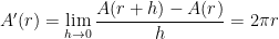
In this series of posts, I’ll discuss several ways that the area of a circle can be found using calculus. I’ll also discuss a straightforward classroom activity by which students can discover for themselves why . In the first few weeks after a calculus class, after students are introduced to the concept of limits, the derivative is introduced for the first time… often as the slope of a tangent line to the curve. Here it is: if $y = f(x)$, then

From this definition, the first few rules of differentiation are derived in approximately the following order:
1. If  , a constant, then
  .
.
2. If  and
and  are both differentiable, then
  .
.
3. If is differentiable and  is a constant, then
  .
.
4. If  , where
  is a nonnegative integer, then
  . This may be proved by at least two different techniques:
- The binomial expansion

- The Product Rule (derived later) and mathematical induction
5. If  is a polynomial, then
  . In other words, taking the derivative of a polynomial is easy.
After doing a few examples to help these concepts sink in, I’ll show the following two examples with about 3-4 minutes left in class.
Example 1. Let  . Notice I’ve changed the variable from
  to
to  , but that’s OK. Does this remind you of anything? (Students answer: the area of a circle.) What’s the derivative? Remember,
  is just a constant. So
 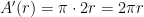 . Does this remind you of anything? (Students answer: Whoa… the circumference of a circle.)
Example 2. Now let’s try  . Does this remind you of anything? (Students answer: the volume of a sphere.) What’s the derivative? Again,
  is just a constant. So
  . Does this remind you of anything? (Students answer: Whoa… the surface area of a sphere.)
Hmmm. That’s interesting. The derivative of the area of a circle is the circumference of the circle, and the derivative of the area of a sphere is the surface area of the sphere. I wonder why this works. Any ideas? (Students: stunned silence.)
This is what’s known on television as a cliff-hanger, and I’ll give you the answer at the start of class tomorrow. (Students groan, as they really want to know the answer immediately.)
In the spirit of a cliff-hanger, I offer the following thought bubble before presenting the answer.

By definition, if , then
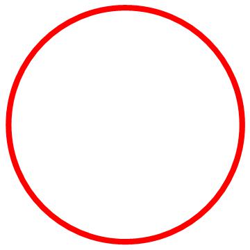
The numerator may be viewed as the area of the ring between concentric circles with radii and  . In other words, imagine starting with a solid red disk of radius
  and then removing a solid white disk of radius . The picture would look something like this:
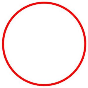
Notice that the ring has a thickness of  . If this ring were to be “unpeeled” and flattened, it would approximately resemble a rectangle. The height of the rectangle would be
  , while the length of the rectangle would be the circumference of the circle. So

and we can conclude that

By the same reasoning, the derivative of the volume of a sphere ought to be the surface area of the sphere.
Pedagogically, I find that the above discussion helps reinforce the definition of a derivative at a time when students are most willing to forget about the formal definition in favor of the various rules of differentiation.
In the above work, we started with the formula for the area of the circle and then confirmed that its derivative matched the expected result. However, the above logic can be used to derive the formula for the area of a circle from the formula $C(r) = 2\pi r$ for the circumference. We begin with the observation that  , as above. Therefore, by the Fundamental Theorem of Calculus,


![A(r) - A(0) = \displaystyle \left[ \pi t^2 \right]_0^r](https://s0.wp.com/latex.php?latex=A%28r%29+-+A%280%29+%3D+%5Cdisplaystyle+%5Cleft%5B+%5Cpi+t%5E2+%5Cright%5D_0%5Er&bg=ffffff&fg=000000&s=0&c=20201002)

Since the area of a circle with radius  is , we conclude that .
Pedagogically, I don’t particularly recommend this approach, as I think students would find this explanation more confusing than the first approach. However, I can see that this could be useful for reinforcing the statement of the Fundamental Theorem of Calculus.
By the way, the above reasoning works for a square or cube also, but with a little twist. For a square of side length  , the area is
  and the perimeter is
  , which isn’t the derivative of
  . The reason this didn’t work is because the side length of a square corresponds to the diameter of a circle, not the radius of a circle.
But, if we let denote half the side length of a square, then the above logic works out since
and

Written in terms of the half-sidelength , we see that  .
.


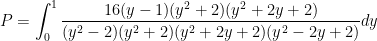
 , so that
  and
and  :
:


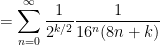
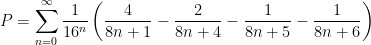
 in the denominator, this infinite series converges very quickly.
 , then we calculate the integral
  , defined below:

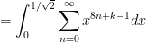

![= \displaystyle \sum_{n=0}^\infty \left[ \frac{x^{8n+k}}{8n+k} \right]^{1/\sqrt{2}}_0](https://s0.wp.com/latex.php?latex=%3D+%5Cdisplaystyle+%5Csum_%7Bn%3D0%7D%5E%5Cinfty+%5Cleft%5B+%5Cfrac%7Bx%5E%7B8n%2Bk%7D%7D%7B8n%2Bk%7D+%5Cright%5D%5E%7B1%2F%5Csqrt%7B2%7D%7D_0&bg=ffffff&fg=000000&s=0&c=20201002)
![= \displaystyle \sum_{n=0}^\infty \frac{1}{8n+k} \left[ \left( \frac{1}{\sqrt{2}} \right)^{8n+k} - 0 \right]](https://s0.wp.com/latex.php?latex=%3D+%5Cdisplaystyle+%5Csum_%7Bn%3D0%7D%5E%5Cinfty+%5Cfrac%7B1%7D%7B8n%2Bk%7D+%5Cleft%5B+%5Cleft%28+%5Cfrac%7B1%7D%7B%5Csqrt%7B2%7D%7D+%5Cright%29%5E%7B8n%2Bk%7D+-+0+%5Cright%5D&bg=ffffff&fg=000000&s=0&c=20201002)
 :
:
 .
. :
:


 Unleashed (Springer, New York, 2000):
 between
  and
and  .
. . With ten rectangles, the approximation is
  . With one hundred rectangles (and Microsoft Excel), the approximation is
  . This last expression was found by evaluating
![0.01[ (0.01)^2 + (0.02)^2 + \dots + (0.99)^2 + 1^2]](https://s0.wp.com/latex.php?latex=0.01%5B+%280.01%29%5E2+%2B+%280.02%29%5E2+%2B+%5Cdots+%2B+%280.99%29%5E2+%2B+1%5E2%5D&bg=ffffff&fg=000000&s=0&c=20201002)
 . And so I’d feel comfortable showing my students the contents of this post. However, if I didn’t know for sure that my students had at least seen this formula, I probably would just ask them to guess the limiting answer without doing any of the algebra to follow.
 . The heights of the rectangles take a little more work to determine. I’ll usually work left to right. The left-most rectangle has right-most
  coordinate of
  . The next rectangle has a height of
  , and so we must evaluate
![\displaystyle \frac{1}{n} \left[ \frac{1^2}{n^2} + \frac{2^2}{n^2} + \dots + \frac{n^2}{n^2} \right]](https://s0.wp.com/latex.php?latex=%5Cdisplaystyle+%5Cfrac%7B1%7D%7Bn%7D+%5Cleft%5B+%5Cfrac%7B1%5E2%7D%7Bn%5E2%7D+%2B+%5Cfrac%7B2%5E2%7D%7Bn%5E2%7D+%2B+%5Cdots+%2B+%5Cfrac%7Bn%5E2%7D%7Bn%5E2%7D+%5Cright%5D&bg=ffffff&fg=000000&s=0&c=20201002) , or
, or![\displaystyle \frac{1}{n^3} \left[ 1^2 + 2^2 + \dots + n^2 \right]](https://s0.wp.com/latex.php?latex=%5Cdisplaystyle+%5Cfrac%7B1%7D%7Bn%5E3%7D+%5Cleft%5B+1%5E2+%2B+2%5E2+%2B+%5Cdots+%2B+n%5E2+%5Cright%5D&bg=ffffff&fg=000000&s=0&c=20201002)
 , or
, or  .
. ,
,  , and
, and  .
. is an example of a rational function, and so the horizontal asymptote can be immediately determined by dividing the leading coefficients of the numerator and denominator (since both have degree 2). We conclude that the limit is
  , and so that’s the area under the parabola.
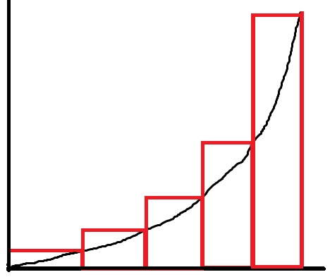
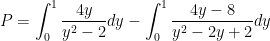
 , but the length takes a little bit more thought. And I make my students figure it out without me giving them the answer. Eventually, someone notices that the height is simply
  , so that the rightmost rectangle has an area of
  .
. . So the area is
  .
. . Students can easily see that this is a decent approximation to the area under the parabola, but it’s a bit too large.
![0.1 [ (0.1)^2 + (0.2)^2 + \dots + (0.9)^2 + 1^2] = 0.385](https://s0.wp.com/latex.php?latex=0.1+%5B+%280.1%29%5E2+%2B+%280.2%29%5E2+%2B+%5Cdots+%2B+%280.9%29%5E2+%2B+1%5E2%5D+%3D+0.385&bg=ffffff&fg=000000&s=0&c=20201002)
 rectangles, the class quickly sees that the sum of the rectangles is
![0.01 [ (0.01)^2 + (0.02)^2 + \dots + (0.99)^2 +( 1.00)^2] = 0.33835](https://s0.wp.com/latex.php?latex=0.01+%5B+%280.01%29%5E2+%2B+%280.02%29%5E2+%2B+%5Cdots+%2B+%280.99%29%5E2+%2B%28+1.00%29%5E2%5D+%3D+0.33835&bg=ffffff&fg=000000&s=0&c=20201002)
 denotes a circular region with radius
  centered at the origin, then
 to
to  , while the angle varies from
  to
to  . Using the
  , we see that
![A = \displaystyle \int_0^{2\pi} \left[ \frac{r^2}{2} \right]_0^a \, d\theta](https://s0.wp.com/latex.php?latex=A+%3D+%5Cdisplaystyle+%5Cint_0%5E%7B2%5Cpi%7D+%5Cleft%5B+%5Cfrac%7Br%5E2%7D%7B2%7D+%5Cright%5D_0%5Ea+%5C%2C+d%5Ctheta&bg=ffffff&fg=000000&s=0&c=20201002)


![[0,2\pi]](https://s0.wp.com/latex.php?latex=%5B0%2C2%5Cpi%5D&bg=ffffff&fg=000000&s=0&c=20201002) and not
and not ![[0^o, 360^o]](https://s0.wp.com/latex.php?latex=%5B0%5Eo%2C+360%5Eo%5D&bg=ffffff&fg=000000&s=0&c=20201002) .
. and
and  . These two functions intersect at
  and
and  . Therefore, the area of the circle is the integral of the difference of the two functions:
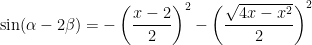
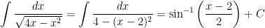
![A = \displaystyle \int_{-r}^r \left[g(x) - f(x) \right] \, dx= \displaystyle \int_{-r}^r 2 \sqrt{r^2 - x^2} \, dx](https://s0.wp.com/latex.php?latex=A+%3D+%5Cdisplaystyle+%5Cint_%7B-r%7D%5Er+%5Cleft%5Bg%28x%29+-+f%28x%29+%5Cright%5D+%5C%2C+dx%3D+%5Cdisplaystyle+%5Cint_%7B-r%7D%5Er+2+%5Csqrt%7Br%5E2+-+x%5E2%7D+%5C%2C+dx&bg=ffffff&fg=000000&s=0&c=20201002)
 and changing the range of integration to
  to
to  . Since
  , we find


![A = \displaystyle r^2 \left[ \theta + \frac{1}{2} \sin 2\theta \right]_{-\pi/2}^{\pi/2}](https://s0.wp.com/latex.php?latex=A+%3D+%5Cdisplaystyle+r%5E2+%5Cleft%5B+%5Ctheta+%2B+%5Cfrac%7B1%7D%7B2%7D+%5Csin+2%5Ctheta+%5Cright%5D_%7B-%5Cpi%2F2%7D%5E%7B%5Cpi%2F2%7D&bg=ffffff&fg=000000&s=0&c=20201002)
![A = \displaystyle r^2 \left[ \left( \displaystyle \frac{\pi}{2} + \frac{1}{2} \sin \pi \right) - \left( - \frac{\pi}{2} + \frac{1}{2} \sin (-\pi) \right) \right]](https://s0.wp.com/latex.php?latex=A+%3D+%5Cdisplaystyle+r%5E2+%5Cleft%5B+%5Cleft%28+%5Cdisplaystyle+%5Cfrac%7B%5Cpi%7D%7B2%7D+%2B+%5Cfrac%7B1%7D%7B2%7D+%5Csin+%5Cpi+%5Cright%29+-+%5Cleft%28+-+%5Cfrac%7B%5Cpi%7D%7B2%7D+%2B+%5Cfrac%7B1%7D%7B2%7D+%5Csin+%28-%5Cpi%29+%5Cright%29+%5Cright%5D&bg=ffffff&fg=000000&s=0&c=20201002)
![[-\pi/2,\pi/2]](https://s0.wp.com/latex.php?latex=%5B-%5Cpi%2F2%2C%5Cpi%2F2%5D&bg=ffffff&fg=000000&s=0&c=20201002) and not
and not ![[-90^o, 90^o]](https://s0.wp.com/latex.php?latex=%5B-90%5Eo%2C+90%5Eo%5D&bg=ffffff&fg=000000&s=0&c=20201002) .
.