In this series of posts, I provide a deeper look at common applications of exponential functions that arise in an Algebra II or Precalculus class. In the previous posts in this series, I considered financial applications, radioactive decay, and Newton’s Law of Cooling.
Today, I introduce the logistic growth model, which describes how an infection (like a disease, a rumor, or advertise) spreads in a population. Before I actually present the formula to my students, I usually perform a 8- to 10-minute demonstration to convince students that the formula actually works. This demonstration works well with between 15 and 45 students; I have personally not attempted this demo with a class larger than 45.
I wish I could take credit for the idea behind this demonstration. I’m afraid I can’t remember who told me the idea behind this demo about 15 years ago, but I’m thankful to him or her for this idea, as I’ve used it with great success over the years when teaching Precalculus and even when teaching Differential Equations.
Here’s the demonstration:
1. The class period before the demo, I ask my students to bring their calculators to class.
2. On the day of the demo, I prepare slips of paper with the numbers 1, 2, 3, etc. I hand these to my students as they take their seats before class starts (and, as needed, to students who arrive late).
3. I tell the class that we’re going to model how a rumor gets spread. On the chalkboard, I write down the numbers 0, 1, 2, …, up to  , the number of students in the class that day. Invariably, I get asked, “What’s the rumor?” In response, I’ll playfully point to someone in the front row and say, “The rumor is about him.”
4. I point out that, at time 0, only one person has heard the rumor…. me. I’m person number 0 (confirming the popular belief of my students). So I’ll cross out the 0 on the board and mark on a table that only one person has heard the rumor so far. (Here’s the spreadsheet that I’ve used to keep track of this information while simultaneously making a graph of the data: logisitic).
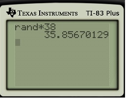
5. I begin to spread the rumor. To spread the rumor, I use my calculator to get a random number between  and . This can be done by just using the built-in random number generator found on many calculators and then multiplying by
  . (After all, there are
  people in the room: students plus one instructor.) The part after the decimal point is not important; the number before the decimal point represents the next person to hear the rumor.
For example, in the figure below, I would tell that person #35 of my class of 37 students was the next to hear the rumor. (If my random number is 0, I’ll privately cheat and get until I get a random number other than 0. I only permit the possibility of cheating on the first step so that the data fits the predicted curve as accurately as possible.)
 6. At this point, I’ll X out the number of the next person to hear the rumor (in this case, 35), and I then ask how many people have heard the rumor. Obviously, two people have heard the rumor. So I’ll note on the table that two people have heard the rumor after one step.
7. Now we repeat the process. I get a new random number, and I ask the first student to pull out his/her calculator to get a random number too. But there’s an important rule: if you get a number that’s already been called, that’s OK. This models what really happens when a rumor (or disease) spreads in a population — it’s perfectly possible to hear the rumor twice.
8. We repeat the process — X’ing out numbers that have been previously called and students calling out the next person to hear the rumor — until the entire class hears the rumor. At some point, it becomes easiest to ask students to only call out if they get a number that hasn’t been called yet. Invariably, there’s always one person at the end who hasn’t heard the rumor yet, and this student is often the subject of some good-natured ribbing. Eventually, a chart like the following is produced.

9. Students immediately see that this is a different type of function than pure exponential growth. It actually does start off looking like exponential growth, but at some point the curve levels off. This makes sense because there’s a limiting value of  (in this case, 38), which can’t happen for a model like
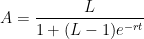
10. The punchline is that the spreadsheet secretly computes the actual curve predicted by the logistic growth model. The numbers are actually located in column C, which is conveniently hidden beneath the graph. The function is
 ,
,
where  . (Had each person the rumor to two different people at each step, then
  would have been equal to
  .) Here’s the graph, superimposed upon the data collected from class. I can do this pretty quickly in class because the curve is actually already drawn in the figure above… but it’s drawn in gray, the same color as the background. By changing the color to black, the graph becomes clear:

I never expect the curve to exactly fit the data, but it should come pretty close. After this fairly dramatic revelation, my students are completely sold that the mathematics that I’m about to show them actually works.


![A(t) [ L - A(t) ]](https://s0.wp.com/latex.php?latex=A%28t%29+%5B+L+-+A%28t%29+%5D+&bg=ffffff&fg=000000&s=0&c=20201002)
![A'(t) = c A(t) [ L - A(t) ]](https://s0.wp.com/latex.php?latex=A%27%28t%29+%3D+c+A%28t%29+%5B+L+-+A%28t%29+%5D&bg=ffffff&fg=000000&s=0&c=20201002)


![A'(t) = \displaystyle \frac{r}{L} A(t) [ L - A(t) ]](https://s0.wp.com/latex.php?latex=A%27%28t%29+%3D+%5Cdisplaystyle+%5Cfrac%7Br%7D%7BL%7D+A%28t%29+%5B+L+-+A%28t%29+%5D&bg=ffffff&fg=000000&s=0&c=20201002)
![A'(t) = r A(t) \displaystyle \left[1 - \frac{A(t)}{L} \right]](https://s0.wp.com/latex.php?latex=A%27%28t%29+%3D+r+A%28t%29+%5Cdisplaystyle+%5Cleft%5B1+-+%5Cfrac%7BA%28t%29%7D%7BL%7D+%5Cright%5D&bg=ffffff&fg=000000&s=0&c=20201002)


 of the object is found to be
 ,
, is the time,
  is the constant surrounding temperature, and
  is a constant that depends on the object.
 as a function of time, use linear regression to solve for the constant
  , we find that
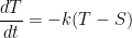 ,
,


 , a number that must be given in the problem:


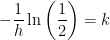
 be the half-life of the substance. By definition, this means that


![A = A_0 e^{ -\left[ -\frac{1}{h} \ln \left( \frac{1}{2} \right) \right] t}](https://s0.wp.com/latex.php?latex=A+%3D+A_0+e%5E%7B+-%5Cleft%5B+-%5Cfrac%7B1%7D%7Bh%7D+%5Cln+%5Cleft%28+%5Cfrac%7B1%7D%7B2%7D+%5Cright%29+%5Cright%5D+t%7D&bg=ffffff&fg=000000&s=0&c=20201002)
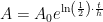
![A = A_0 \left[e^{\ln \left( \frac{1}{2} \right)} \right]^{t/h}](https://s0.wp.com/latex.php?latex=A+%3D+A_0+%5Cleft%5Be%5E%7B%5Cln+%5Cleft%28+%5Cfrac%7B1%7D%7B2%7D+%5Cright%29%7D+%5Cright%5D%5E%7Bt%2Fh%7D&bg=ffffff&fg=000000&s=0&c=20201002)
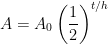
 has been replaced by a new base of
  . For most applications, a base of


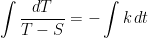
 of a radioactive substance (carbon-14, uranium-235, brain cells) is present, the rate at which the substance decays is proportional to the amount of the substance currently present. This can be rewritten as a differential equation, since the rate at which the substance decays is
  . So we find that


 , a number that must be given in the problem:


 ,
,  , and
, and  , the amount left on the credit card after
 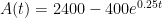 .
.
 Under the theory that a picture is worth a thousand words, let’s take a look at the graphs of both of these functions:
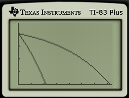

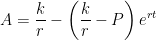
 , has solution
 is the initial amount,
  years to pay off the debt.
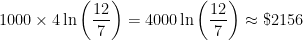
 per year for
  years, and so the amount spent is
 .
.
 :
:

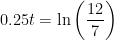


 .
. per year.
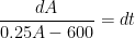


 , we use the initial condition


 with solution
  . The meaning of the value of
  are
are  , while the units of
  . Therefore, the units of
  . So saying that there’s a “relative rate of growth of 10% per hour” makes total sense.
 .” But this is a horrible way to write this in ordinary English! After all, if we plug
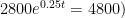
  into the formula, we obtain


