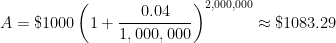
In the previous series of posts, I consider how two different definitions of a logarithmic function are actually related to each other. In this series of posts, I consider how two different definitions of the number  are related to each other.
The number is usually introduced at two different places in the mathematics curriculum:
- Algebra II/Precalculus: If
 dollars are invested at interest rate
  for
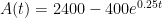
for  years with continuous compound interest, then the amount of money after years is
  .
.
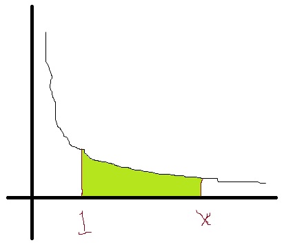
- Calculus: The number is defined to be the number so that the area under the curve
 from
from  to
to  is equal to
  , so that
 .
.
These two definitions appear to be very, very different. One deals with making money. The other deals with the area under a hyperbola. Amazingly, these two definitions are related to each other. In this series of posts, I’ll discuss the connection between the two.
I should say at the outset that the second definition is usually considered the true definition of . However, compound interest usually appears earlier in the mathematics curriculum than definite integrals, and so an informal definition of is given at that stage of the curriculum.


I begin this series of posts with a justification for the compound interest formula  when interest is compounded
  times a year. My experience is that most math majors are familiar with this formula from their high school experience but have absolutely no idea about why it is true, and so the presentation below fills in a major hole in their preparation to become secondary teachers themselves.
In the near future, I’ll discuss how the above formula naturally leads to the formula  when interest is continuously compounded.
I start with a sequence of numerical examples.
A. Suppose that you invest $1,000 at 4% interest for 2 years. (At the time of this writing, a fixed interest rate of 4% is almost mythological, but let’s leave that aside for the sake of the problem.) How much money do you have if the money is compounded annually? Here are the brute force steps. (To make the presentation less dry, I make sure that my students are volunteering each answer before proceeding to the next step.)
- Amount of interest earned in Year 1 =
 .
.
- Total amount of money after Year 1 =
 .
.
- Amount of interest earned in Year 2 =
 .
.
- Total amount of money earned in Year 2 =
 .
.
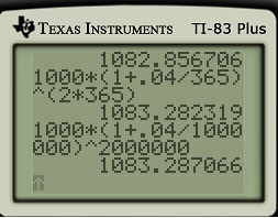
B. Let’s repeat the above problem, except this time the 4% interest is compounded twice a year. In other words, 2% interest is applied every six months.
- Amount of interest earned in first six months =
 .
.
- Total amount of money after first six months =
 .
.
- Amount of interest earned in second six months =
 .
.
- Total amount of money earned after second six months =
 .
.
At this point, I’ll make a big production about how much work this is, and we’re only halfway done with this calculation! So, I’ll rhetorically ask my class, is there an easier way to do this? Let’s take a look back at the first calculation, adding some observations.
- Amount of interest earned in Year 1 =
 .
.
- Total amount of money after Year 1 =
 .
.
- Amount of interest earned in Year 2 =
 .
.
- Total amount of money earned in Year 2 =

 .
.
Then I’ll check with a calculator to confirm that  is indeed equal to
  .
.
Let’s now return to the problem when the 4% interest is compounded twice a year. We’re only halfway through the calculation, but let’s recapitulate what we’ve done so far. Since this is very similar to the above work, students usually can produce the logic very quickly.
- Amount of interest earned in first six months =
 .
.
- Total amount of money after first six months =
 .
.
- Amount of interest earned in second six months =
 .
.
- Total amount of money earned after second six months =
 .
.
 .
.
At this point, I’ll ask my class what they think how much money will accumulate after two years. Invariably, they guess the correct answer of $latex $1000(1+0.02)^4$. If my class seems to get it, I usually will just accept this as the correct answer without explicitly running through steps 5 through 8 to get to the end of the fourth six weeks.
C. What is the money makes 4% interest compounded four times a year for 2 years? By this point, my students can usually guess the answer:  . The
. The  comes from dividing the 4% into four parts. The 8 comes from the number of compounding periods over 2 years.
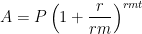
D. By this point, we have pretty much arrived at the compound interest formula:  . The above argument justifies the formula; the actual proof of the formula is very similar to the above numerical examples, and so I don’t use class time to formally prove it.
Tomorrow, I’ll give some pedagogical thoughts about these computations.


per year.
per year.


 with solution
  are
are  , while the units of
  . Therefore, the units of
  . So saying that there’s a “relative rate of growth of 10% per hour” makes total sense.
 .” But this is a horrible way to write this in ordinary English! After all, if we plug
  into the formula, we obtain


 . In today’s post, I’d like to give the more formal derivation using calculus.
 should earn ten times as much interest as
  . Since


 , with the understanding that
  ).
). :
:


 .
. as
as  .
. instead of
  . In this way, we can think like an
  . Then the discrete compound interest formula becomes

![A = P\displaystyle \left[ \left( 1 + \frac{1}{m} \right)^m \right]^{rt}](https://s0.wp.com/latex.php?latex=A+%3D+P%5Cdisplaystyle+%5Cleft%5B+%5Cleft%28+1+%2B+%5Cfrac%7B1%7D%7Bm%7D+%5Cright%29%5Em+%5Cright%5D%5E%7Brt%7D&bg=ffffff&fg=000000&s=0&c=20201002)
 , except that the name of the variable has changed from
  . But that’s no big deal: as
  and both
 ,
, , so that we can simply replace
  increases as
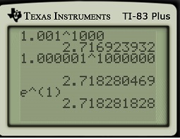
  ) that earns 100% interest (so that
  ) for one year (so that
 , then
  . I’ll usually double-check with my class to make sure that they believe this answer… that $1 compounded once at 100% interest results in $2.
 , then
 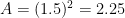 .
. , then
  .
. , then
  .
. , then
 , then
 treatment of limit in an honors calculus class or in real analysis. So, mathematically speaking, the above argument should not be considered a proper definition of the number
  .
. .
. .
. ). Then
  .
. .
.
 , and so the annual percentage rate would really be 26.824%.
 a few times and see if a pattern can be developed. However, my observation is that college students have no memory of being taught how the compound interest formula
 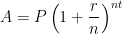 can be seen as a natural consequence of the simple interest formula. In other words, they’d just use the compound interest formula without having any conceptual understanding of where the formula came from.
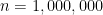
 . What is the probability that, after playing
  . Therefore, the chance of not winning
  , which we can approximate with a calculator.
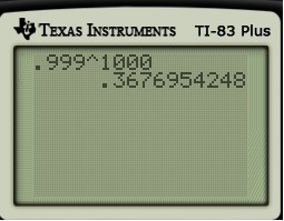

 ? Then the probability would be
  .
.
 .
.
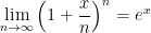
 , we find
 , we have
![\ln \left[ \displaystyle \lim_{n \to \infty} \left(1 + \frac{x}{n}\right)^n \right] = \displaystyle \lim_{n \to \infty} \ln \left[ \left(1 + \frac{x}{n}\right)^n \right]](https://s0.wp.com/latex.php?latex=%5Cln+%5Cleft%5B+%5Cdisplaystyle+%5Clim_%7Bn+%5Cto+%5Cinfty%7D+%5Cleft%281+%2B+%5Cfrac%7Bx%7D%7Bn%7D%5Cright%29%5En+%5Cright%5D+%3D+%5Cdisplaystyle+%5Clim_%7Bn+%5Cto+%5Cinfty%7D+%5Cln+%5Cleft%5B+%5Cleft%281+%2B+%5Cfrac%7Bx%7D%7Bn%7D%5Cright%29%5En+%5Cright%5D&bg=ffffff&fg=000000&s=0&c=20201002)
![\ln \left[ \displaystyle \lim_{n \to \infty} \left(1 + \frac{x}{n}\right)^n \right] = \displaystyle \lim_{n \to \infty} n \ln \left(1 + \frac{x}{n}\right)](https://s0.wp.com/latex.php?latex=%5Cln+%5Cleft%5B+%5Cdisplaystyle+%5Clim_%7Bn+%5Cto+%5Cinfty%7D+%5Cleft%281+%2B+%5Cfrac%7Bx%7D%7Bn%7D%5Cright%29%5En+%5Cright%5D+%3D+%5Cdisplaystyle+%5Clim_%7Bn+%5Cto+%5Cinfty%7D+n+%5Cln+%5Cleft%281+%2B+%5Cfrac%7Bx%7D%7Bn%7D%5Cright%29&bg=ffffff&fg=000000&s=0&c=20201002)
![\ln \left[ \displaystyle \lim_{n \to \infty} \left(1 + \frac{x}{n}\right)^n \right] = \displaystyle \lim_{n \to \infty} \frac{ \displaystyle \ln \left(1 + \frac{x}{n}\right)}{\displaystyle \frac{1}{n}}](https://s0.wp.com/latex.php?latex=%5Cln+%5Cleft%5B+%5Cdisplaystyle+%5Clim_%7Bn+%5Cto+%5Cinfty%7D+%5Cleft%281+%2B+%5Cfrac%7Bx%7D%7Bn%7D%5Cright%29%5En+%5Cright%5D+%3D+%5Cdisplaystyle+%5Clim_%7Bn+%5Cto+%5Cinfty%7D+%5Cfrac%7B+%5Cdisplaystyle+%5Cln+%5Cleft%281+%2B+%5Cfrac%7Bx%7D%7Bn%7D%5Cright%29%7D%7B%5Cdisplaystyle+%5Cfrac%7B1%7D%7Bn%7D%7D&bg=ffffff&fg=000000&s=0&c=20201002)
 as
as  , and so we may use L’Hopital’s rule, differentiating both the numerator and the denominator with respect to
 ![\ln \left[ \displaystyle \lim_{n \to \infty} \left(1 + \frac{x}{n}\right)^n \right] = \displaystyle \lim_{n \to \infty} \frac{ \displaystyle \frac{1}{1 + \frac{x}{n}} \cdot \frac{-x}{n^2} }{\displaystyle \frac{-1}{n^2}}](https://s0.wp.com/latex.php?latex=%5Cln+%5Cleft%5B+%5Cdisplaystyle+%5Clim_%7Bn+%5Cto+%5Cinfty%7D+%5Cleft%281+%2B+%5Cfrac%7Bx%7D%7Bn%7D%5Cright%29%5En+%5Cright%5D+%3D+%5Cdisplaystyle+%5Clim_%7Bn+%5Cto+%5Cinfty%7D+%5Cfrac%7B+%5Cdisplaystyle+%5Cfrac%7B1%7D%7B1+%2B+%5Cfrac%7Bx%7D%7Bn%7D%7D+%5Ccdot+%5Cfrac%7B-x%7D%7Bn%5E2%7D+%7D%7B%5Cdisplaystyle+%5Cfrac%7B-1%7D%7Bn%5E2%7D%7D&bg=ffffff&fg=000000&s=0&c=20201002)
![\ln \left[ \displaystyle \lim_{n \to \infty} \left(1 + \frac{x}{n}\right)^n \right] = \displaystyle \lim_{n \to \infty} \displaystyle \frac{x}{1 + \frac{x}{n}}](https://s0.wp.com/latex.php?latex=%5Cln+%5Cleft%5B+%5Cdisplaystyle+%5Clim_%7Bn+%5Cto+%5Cinfty%7D+%5Cleft%281+%2B+%5Cfrac%7Bx%7D%7Bn%7D%5Cright%29%5En+%5Cright%5D+%3D+%5Cdisplaystyle+%5Clim_%7Bn+%5Cto+%5Cinfty%7D+%5Cdisplaystyle+%5Cfrac%7Bx%7D%7B1+%2B+%5Cfrac%7Bx%7D%7Bn%7D%7D&bg=ffffff&fg=000000&s=0&c=20201002)
![\ln \left[ \displaystyle \lim_{n \to \infty} \left(1 + \frac{x}{n}\right)^n \right] = \displaystyle \frac{x}{1 + 0}](https://s0.wp.com/latex.php?latex=%5Cln+%5Cleft%5B+%5Cdisplaystyle+%5Clim_%7Bn+%5Cto+%5Cinfty%7D+%5Cleft%281+%2B+%5Cfrac%7Bx%7D%7Bn%7D%5Cright%29%5En+%5Cright%5D+%3D+%5Cdisplaystyle+%5Cfrac%7Bx%7D%7B1+%2B+0%7D&bg=ffffff&fg=000000&s=0&c=20201002)
![\ln \left[ \displaystyle \lim_{n \to \infty} \left(1 + \frac{x}{n}\right)^n \right] = x](https://s0.wp.com/latex.php?latex=%5Cln+%5Cleft%5B+%5Cdisplaystyle+%5Clim_%7Bn+%5Cto+%5Cinfty%7D+%5Cleft%281+%2B+%5Cfrac%7Bx%7D%7Bn%7D%5Cright%29%5En+%5Cright%5D+%3D+x&bg=ffffff&fg=000000&s=0&c=20201002)


 ,
,  ,
,  , and
, and  .
. .
.

 and that


 minutes) there will be 5400 bacteria.
 and the student must solve for
  . The first “hint” the website provides is “look at the bases. Rewrite them as a common base” and then the website shows them the work. The student will continue hitting the “next” button until all steps are complete. This is allowing the visual learners to see how to write out each step to successfully complete the problem.