I recently finished the novel Shantaram, by Gregory David Roberts. As I’m not a professional book reviewer, let me instead quote from the Amazon review:
Crime and punishment, passion and loyalty, betrayal and redemption are only a few of the ingredients in Shantaram, a massive, over-the-top, mostly autobiographical novel. Shantaram is the name given Mr. Lindsay, or Linbaba, the larger-than-life hero. It means “man of God’s peace,” which is what the Indian people know of Lin. What they do not know is that prior to his arrival in Bombay he escaped from an Australian prison where he had begun serving a 19-year sentence. He served two years and leaped over the wall. He was imprisoned for a string of armed robberies performed to support his heroin addiction, which started when his marriage fell apart and he lost custody of his daughter. All of that is enough for several lifetimes, but for Greg Roberts, that’s only the beginning.
He arrives in Bombay with little money, an assumed name, false papers, an untellable past, and no plans for the future. Fortunately, he meets Prabaker right away, a sweet, smiling man who is a street guide. He takes to Lin immediately, eventually introducing him to his home village, where they end up living for six months. When they return to Bombay, they take up residence in a sprawling illegal slum of 25,000 people and Linbaba becomes the resident “doctor.” With a prison knowledge of first aid and whatever medicines he can cadge from doing trades with the local Mafia, he sets up a practice and is regarded as heaven-sent by these poor people who have nothing but illness, rat bites, dysentery, and anemia. He also meets Karla, an enigmatic Swiss-American woman, with whom he falls in love. Theirs is a complicated relationship, and Karla’s connections are murky from the outset.
While it was a cracking good read, what struck me particularly were the surprising mathematical allusions that the author used throughout the novel. In this mini-series, I’d like to explore the ones that I found.

In this first installment, the narrator describes a life-or-death situation as he is being choked:
He was a hard man. He didn’t give up. His hands squeezed tighter. My neck was strong and the muscles were well developed, but I knew he had the strength to kill me. My hand reached, groping for the pistol in my pocket. I had to shoot him. I had to kill him. That was all right. I didn’t care. The air in my lungs was spent, and my brain was exploding in Mandelbrot whirls of colored light, and I was dying, and I wanted to kill him.
Shantaram, Chapter 25
Someone being choked to death might be prosaically described as “seeing stars,” but the author instead to choose the more vivid imagery of “exploding in Mandelbrot whirls of colored light.” The Mandelbrot set is a fractal that solves a famous mathematical problem:
And the Mandelbrot set is quite colorful and complex, which might indeed be a better description than “seeing stars” of what might be going through someone’s mind when being choked to death. Although somewhat dated, here’s my favorite Mandelbrot zoom video:
 and
and 
 ,
,  , and
, and  near
near  (or, more generally, their Taylor series approximations)
 substitution
 th order homogeneous differential equation with constant coefficients
 ,
,
 determines the solutions of the differential equation.
 . Differentiating, we find
  ,
,  , etc. Therefore, the differential equation becomes


 can never be equal to
  . Therefore, solving the differential equation reduces to finding the roots of this polynomial, which can be done using standard techniques from Precalculus.
 . The characteristic equation is
  , which has roots
  . Therefore, two solutions to the differential equation are
  and
and  , so that the general solution is
 .
. , so that


 .
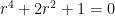
. . To find the roots of the characteristic equation, we factor:


 .
. , and
, and  , so that the general solution is
 .
. .
. with the Sun at the origin, under general relativity follows the initial-value problem
  ,
, ,
, ,
, ,
,  ,
,  ,
,  is the gravitational constant of the universe,
  is the mass of the planet,
  is the mass of the Sun,
  is the constant angular momentum of the planet,
  is the speed of light, and
  is the smallest distance of the planet from the Sun during its orbit (i.e., at perihelion).
 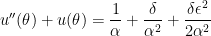 .
. .
. .
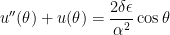
. . Then
  satisfies the new differential equation
  . Also,
  . Substituting, we find


 .
. and
and  can be found by substituting back into the original differential equation:

 and
and  . Therefore, the solution of the simplified differential equation is
 .
. and
and  , we see that

 is some unknown function, to find the general solution of the differential equation
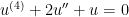 .
.
 .
. . If
. If  , then
 ,
, ,
, ,
, .
.


 and
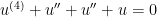
and  cancelled each other. This new differential equation doesn’t look like much of an improvement over the original fourth-order differential equation, but we can make a key observation: if
  , then differentiating twice more trivially yields
  and
and  . Said another way: if

 .
. .
. :
:


 .
. , so that
  . Therefore, another solution of the original differential equation will be
 .
. .
. .
. ,
, .
. , which corresponds to the second-order differential equation
  . We’ve already seen that
  and
and  are solutions of this differential equation; perhaps they might also be solutions of the more complicated differential equation also? The answer, of course, is yes:
 .
. ,
, .
. :
:![(fg)'' = ( [fg]')' = (f'g)' + (fg')'](https://s0.wp.com/latex.php?latex=%28fg%29%27%27+%3D+%28+%5Bfg%5D%27%29%27+%3D+%28f%27g%29%27+%2B+%28fg%27%29%27&bg=ffffff&fg=000000&s=0&c=20201002)

 .
. :
:![(fg)''' = ( [fg]'')' = (f''g)' + 2(f'g')' + (fg'')'](https://s0.wp.com/latex.php?latex=%28fg%29%27%27%27+%3D+%28+%5Bfg%5D%27%27%29%27+%3D+%28f%27%27g%29%27+%2B+2%28f%27g%27%29%27+%2B++%28fg%27%27%29%27&bg=ffffff&fg=000000&s=0&c=20201002)

 .
.![(fg)^{(4)} = ( [fg]''')' = (f'''g)' + 3(f''g')' +3(f'g'')' + (fg''')'](https://s0.wp.com/latex.php?latex=%28fg%29%5E%7B%284%29%7D+%3D+%28+%5Bfg%5D%27%27%27%29%27+%3D+%28f%27%27%27g%29%27+%2B+3%28f%27%27g%27%29%27+%2B3%28f%27g%27%27%29%27+%2B+%28fg%27%27%27%29%27&bg=ffffff&fg=000000&s=0&c=20201002)

 .
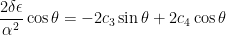
. .
. . Then
  . Since
  , we may substitute:
 . Therefore,
  and
and  are both double roots of this quartic equation. Therefore, the general solution for
  is
is .
.

 and
and  . Therefore,
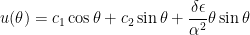
 , we find that
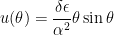
 term is what predicts the precession of a planet’s orbit under general relativity.
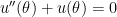
 , with the Sun at the origin, then under Newtonian mechanics (i.e., without general relativity) the motion of the planet follows the differential equation
 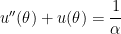 ,
, and
and  is a certain constant. We will also impose the initial condition that the planet is at perihelion (i.e., is closest to the sun), at a distance of
  . This means that
  when
when 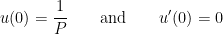 ;
; .
. . Therefore, two linearly independent solutions of the associated homogeneous equation are
  , but complex numbers provide a way of solving the differential equations that model multiple problems in statics and dynamics.)
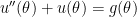
 ,
, ,
, ,
, is the Wronskian of
  and
and  , defined by the determinant
 .
.
 and
and  essentially disappear.
 , the integrals for
  ,
, for the constant of integration instead of the usual
  . Second,
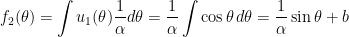 ,
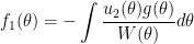
, for the constant of integration. Therefore, by variation of parameters, the general solution of the nonhomogeneous differential equation is
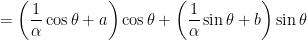
 .
. and
and  . This is require using the initial conditions


 .
.
 ,
, .
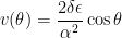
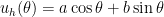
. , we see that the planet’s orbit satisfies
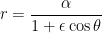 ,
, .
. .
. is not a solution of the characteristic equation, this leads to trying something of the form
  as a solution, where
  is a soon-to-be-determined constant. (Guessing this form of
  is a standard technique from differential equations; later in this series, I’ll give some justification for this guess.)
 and
and  . Substituting, we find


 is a particular solution of the nonhomogeneous differential equation.
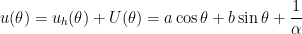 .
.
