The following problem appeared in Volume 97, Issue 3 (2024) of Mathematics Magazine.
Two points  and
and  are chosen at random (uniformly) from the interior of a unit circle. What is the probability that the circle whose diameter is segment
  lies entirely in the interior of the unit circle?
As discussed in a previous post, I guessed from simulation that the answer is  . Naturally, simulation is not a proof, and so I started thinking about how to prove this.
My first thought was to make the problem simpler by letting only one point be chosen at random instead of two. Suppose that the point is fixed at a distance  from the origin. What is the probability that the point , chosen at random, uniformly, from the interior of the unit circle, has the desired property?
My second thought is that, by radial symmetry, I could rotate the figure so that the point is located at  . In this way, the probability in question is ultimately going to be a function of .
There is a very nice way to compute such probabilities since is chosen at uniformly from the unit circle. Let  be the set of all points within the unit circle that have the desired property. Since the area of the unit circle is
  , the probability of desired property happening is
 .
.
Based on the simulations discussed in the previous post, my guess was that was the interior of an ellipse centered at the origin with a semimajor axis of length  and a semiminor axis of length
  . Now I had to think about how to prove this.
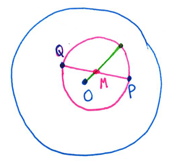
As noted earlier in this series, the circle with diameter  will lie within the unit circle exactly when
  , where
  is the midpoint of . So suppose that has coordinates , where is known, and let the coordinates of be
  . Then the coordinates of will be
 ,
,
so that

and
 .
.
Therefore, the condition (again, equivalent to the condition that the circle with diameter lies within the unit circle) becomes
 ,
,
which simplifies to
![\displaystyle \sqrt{ \frac{1}{4} \left[ (x+t)^2 + y^2 \right]} + \sqrt{ \frac{1}{4} \left[ (x-t)^2 + y^2 \right]} < 1](https://s0.wp.com/latex.php?latex=%5Cdisplaystyle+%5Csqrt%7B+%5Cfrac%7B1%7D%7B4%7D+%5Cleft%5B+%28x%2Bt%29%5E2+%2B+y%5E2+%5Cright%5D%7D+%2B+%5Csqrt%7B+%5Cfrac%7B1%7D%7B4%7D+%5Cleft%5B+%28x-t%29%5E2+%2B+y%5E2+%5Cright%5D%7D+%3C+1&bg=ffffff&fg=000000&s=0&c=20201002)

 .
.
When I saw this, light finally dawned. Given two points  and
and  , called the foci, an ellipse is defined to be the set of all points so that
  , where
  is a constant. If the coordinates of , , and are ,
  , and
, and  , then this becomes
 .
.
Therefore, the set is the interior of an ellipse centered at the origin with  and
and  . Furthermore, is the semimajor axis of the ellipse, while the semiminor axis is equal to
  .
.
At last, I could now return to the original question. Suppose that the point is fixed at a distance from the origin. What is the probability that the point , chosen at random, uniformly, from the interior of the unit circle, has the property that the circle with diameter lies within the unit circle? Since is a subset of the interior of the unit circle, we see that this probability is equal to
 .
.
In the next post, I’ll use this intermediate step to solve the original question.
and
be independent normally distributed random variables, each with its own mean and variance. Show that the variance of
is smaller than the variance of


![\hbox{Var}(X \mid X > Y) = E(X^2 \mid X > Y) - [E(X \mid X > Y)]^2 < \hbox{Var}(X) = \sigma_1^2](https://s0.wp.com/latex.php?latex=%5Chbox%7BVar%7D%28X+%5Cmid+X+%3E+Y%29+%3D+E%28X%5E2+%5Cmid+X+%3E+Y%29+-+%5BE%28X+%5Cmid+X+%3E+Y%29%5D%5E2+%3C+%5Chbox%7BVar%7D%28X%29+%3D+%5Csigma_1%5E2&bg=ffffff&fg=000000&s=0&c=20201002)


 and
and  , where
  could be something other than 1. The goal is to show that
![\hbox{Var}(X \mid X > Y) = E(X^2 \mid X > Y) - [E(X \mid X > Y)]^2 < 1](https://s0.wp.com/latex.php?latex=%5Chbox%7BVar%7D%28X+%5Cmid+X+%3E+Y%29+%3D+E%28X%5E2+%5Cmid+X+%3E+Y%29+-+%5BE%28X+%5Cmid+X+%3E+Y%29%5D%5E2+%3C+1&bg=ffffff&fg=000000&s=0&c=20201002) .
. . The denominator is straightforward: since
  is normally distributed with
  . (Also,
  , but that’s really not needed for this problem.) Therefore,
  since the distribution of
  .
. , where
  has a standard normal distribution. Then
 ,
, , matching the requirement
  . The inner integral can be directly evaluated:
![E(X I_{X>Y}) = \displaystyle \frac{1}{2\pi} \int_{-\infty}^\infty \left[ -e^{-x^2/2} \right]_{\sigma z}^\infty e^{-z^2/2} \, dz](https://s0.wp.com/latex.php?latex=E%28X+I_%7BX%3EY%7D%29+%3D+%5Cdisplaystyle+%5Cfrac%7B1%7D%7B2%5Cpi%7D+%5Cint_%7B-%5Cinfty%7D%5E%5Cinfty+%5Cleft%5B+-e%5E%7B-x%5E2%2F2%7D+%5Cright%5D_%7B%5Csigma+z%7D%5E%5Cinfty+e%5E%7B-z%5E2%2F2%7D+%5C%2C+dz&bg=ffffff&fg=000000&s=0&c=20201002)
![= \displaystyle \frac{1}{2\pi} \int_{-\infty}^\infty \left[ 0 + e^{-\sigma^2 z^2/2} \right] e^{-z^2/2} \, dz](https://s0.wp.com/latex.php?latex=%3D+%5Cdisplaystyle+%5Cfrac%7B1%7D%7B2%5Cpi%7D+%5Cint_%7B-%5Cinfty%7D%5E%5Cinfty+%5Cleft%5B+0+%2B+e%5E%7B-%5Csigma%5E2+z%5E2%2F2%7D+%5Cright%5D+e%5E%7B-z%5E2%2F2%7D+%5C%2C+dz&bg=ffffff&fg=000000&s=0&c=20201002)
 .
.![E(X I_{X>Y}) = \displaystyle \frac{1}{\sqrt{2\pi} \sqrt{\sigma^2+1}} \int_{-\infty}^\infty \frac{1}{\sqrt{2\pi} \sqrt{ \frac{1}{\sigma^2+1}}} \exp \left[ -\frac{z^2}{2 \cdot \frac{1}{\sigma^2+1}} \right] \, dz](https://s0.wp.com/latex.php?latex=E%28X+I_%7BX%3EY%7D%29+%3D+%5Cdisplaystyle+%5Cfrac%7B1%7D%7B%5Csqrt%7B2%5Cpi%7D+%5Csqrt%7B%5Csigma%5E2%2B1%7D%7D+%5Cint_%7B-%5Cinfty%7D%5E%5Cinfty+%5Cfrac%7B1%7D%7B%5Csqrt%7B2%5Cpi%7D+%5Csqrt%7B+%5Cfrac%7B1%7D%7B%5Csigma%5E2%2B1%7D%7D%7D+%5Cexp+%5Cleft%5B+-%5Cfrac%7Bz%5E2%7D%7B2+%5Ccdot+%5Cfrac%7B1%7D%7B%5Csigma%5E2%2B1%7D%7D+%5Cright%5D+%5C%2C+dz&bg=ffffff&fg=000000&s=0&c=20201002) .
. , and so the integral must be equal to 1. We conclude
 .
. .
.
![= \displaystyle \left[-x e^{-x^2/2} \right]_{\sigma z}^\infty + \int_{\sigma z}^\infty e^{-x^2/2} \, dx](https://s0.wp.com/latex.php?latex=%3D+%5Cdisplaystyle+%5Cleft%5B-x+e%5E%7B-x%5E2%2F2%7D+%5Cright%5D_%7B%5Csigma+z%7D%5E%5Cinfty+%2B+%5Cint_%7B%5Csigma+z%7D%5E%5Cinfty+e%5E%7B-x%5E2%2F2%7D+%5C%2C+dx&bg=ffffff&fg=000000&s=0&c=20201002)
 .
.
 .
. is an odd function. The double integral is equal to
  , which we’ve already shown is equal to
  .
.![\hbox{Var}(X \mid X > Y) = E(X^2 \mid X > Y) - [E(X \mid X > Y)]^2 = 1 - \displaystyle \frac{2}{\pi(\sigma^2 + 1)}](https://s0.wp.com/latex.php?latex=%5Chbox%7BVar%7D%28X+%5Cmid+X+%3E+Y%29+%3D+E%28X%5E2+%5Cmid+X+%3E+Y%29+-+%5BE%28X+%5Cmid+X+%3E+Y%29%5D%5E2+%3D+1+-+%5Cdisplaystyle+%5Cfrac%7B2%7D%7B%5Cpi%28%5Csigma%5E2+%2B+1%29%7D&bg=ffffff&fg=000000&s=0&c=20201002) ,
, , we recover the conditional variance found in the first special case.
 is greater than
  : if we’re given that
  to be less than
  .
. , but that’s really not needed for this problem.) Therefore,
  ,
, , taking care of the requirement
  . The inner integral can be directly evaluated:
![E(X I_{X>Y}) = \displaystyle \frac{1}{2\pi} \int_{-\infty}^\infty \left[ -e^{-x^2/2} \right]_x^\infty e^{-y^2/2} \, dy](https://s0.wp.com/latex.php?latex=E%28X+I_%7BX%3EY%7D%29+%3D+%5Cdisplaystyle+%5Cfrac%7B1%7D%7B2%5Cpi%7D+%5Cint_%7B-%5Cinfty%7D%5E%5Cinfty+%5Cleft%5B+-e%5E%7B-x%5E2%2F2%7D+%5Cright%5D_x%5E%5Cinfty+e%5E%7B-y%5E2%2F2%7D+%5C%2C+dy&bg=ffffff&fg=000000&s=0&c=20201002)
![= \displaystyle \frac{1}{2\pi} \int_{-\infty}^\infty \left[ 0 + e^{-y^2/2} \right] e^{-y^2/2} \, dy](https://s0.wp.com/latex.php?latex=%3D+%5Cdisplaystyle+%5Cfrac%7B1%7D%7B2%5Cpi%7D+%5Cint_%7B-%5Cinfty%7D%5E%5Cinfty+%5Cleft%5B+0+%2B+e%5E%7B-y%5E2%2F2%7D+%5Cright%5D+e%5E%7B-y%5E2%2F2%7D+%5C%2C+dy&bg=ffffff&fg=000000&s=0&c=20201002)
 .
. :
:![E(X I_{X>Y}) = \displaystyle \frac{1}{\sqrt{2\pi} \sqrt{2}} \int_{-\infty}^\infty \frac{1}{\sqrt{2\pi} \sqrt{1/2}} \exp \left[ -\frac{y^2}{2 \cdot \frac{1}{2}} \right] \, dy](https://s0.wp.com/latex.php?latex=E%28X+I_%7BX%3EY%7D%29+%3D+%5Cdisplaystyle+%5Cfrac%7B1%7D%7B%5Csqrt%7B2%5Cpi%7D+%5Csqrt%7B2%7D%7D+%5Cint_%7B-%5Cinfty%7D%5E%5Cinfty+%5Cfrac%7B1%7D%7B%5Csqrt%7B2%5Cpi%7D+%5Csqrt%7B1%2F2%7D%7D+%5Cexp+%5Cleft%5B+-%5Cfrac%7By%5E2%7D%7B2+%5Ccdot+%5Cfrac%7B1%7D%7B2%7D%7D+%5Cright%5D+%5C%2C+dy&bg=ffffff&fg=000000&s=0&c=20201002) .
. .
. , matching my initial intuition.
 .
.
![= \displaystyle \left[-x e^{-x^2/2} \right]_y^\infty + \int_y^\infty e^{-x^2/2} \, dx](https://s0.wp.com/latex.php?latex=%3D+%5Cdisplaystyle+%5Cleft%5B-x+e%5E%7B-x%5E2%2F2%7D+%5Cright%5D_y%5E%5Cinfty+%2B+%5Cint_y%5E%5Cinfty+e%5E%7B-x%5E2%2F2%7D+%5C%2C+dx&bg=ffffff&fg=000000&s=0&c=20201002)
 .
.
 .
. is an odd function. The double integral is equal to
 ![\hbox{Var}(X \mid X > Y) = E(X^2 \mid X > Y) - [E(X \mid X > Y)]^2 = 1 - \displaystyle \left( \frac{1}{\sqrt{\pi}} \right)^2 = 1 - \frac{1}{\pi}](https://s0.wp.com/latex.php?latex=%5Chbox%7BVar%7D%28X+%5Cmid+X+%3E+Y%29+%3D+E%28X%5E2+%5Cmid+X+%3E+Y%29+-+%5BE%28X+%5Cmid+X+%3E+Y%29%5D%5E2+%3D+1+-+%5Cdisplaystyle+%5Cleft%28+%5Cfrac%7B1%7D%7B%5Csqrt%7B%5Cpi%7D%7D+%5Cright%29%5E2+%3D+1+-+%5Cfrac%7B1%7D%7B%5Cpi%7D&bg=ffffff&fg=000000&s=0&c=20201002) ,
, 
 be the interior of the circle centered at the origin
  with radius
  . Also, let
  denote the circle with diameter
  be the distance of
  .
. , I will integrate over this conditional probability:
 ,
, is the cumulative distribution function of
  . For
. For  ,
, .
. .
. . Then the endpoints
  and
and  become
  and
and  . Also,
  . Therefore,


![= \displaystyle \frac{2}{3} \left[ u^{3/2} \right]_0^1](https://s0.wp.com/latex.php?latex=%3D+%5Cdisplaystyle+%5Cfrac%7B2%7D%7B3%7D+%5Cleft%5B++u%5E%7B3%2F2%7D+%5Cright%5D_0%5E1&bg=ffffff&fg=000000&s=0&c=20201002)
![=\displaystyle \frac{2}{3}\left[ (1)^{3/2} - (0)^{3/2} \right]](https://s0.wp.com/latex.php?latex=%3D%5Cdisplaystyle++%5Cfrac%7B2%7D%7B3%7D%5Cleft%5B+%281%29%5E%7B3%2F2%7D+-+%280%29%5E%7B3%2F2%7D+%5Cright%5D&bg=ffffff&fg=000000&s=0&c=20201002)
 ,
, .
.
 .
.
 ; as it turned out, it looked like the semiminor axis now had a length of
  .
.
 is a Pythagorean triple, meaning that


 , a very familiar number from trigonometry:
 .
.
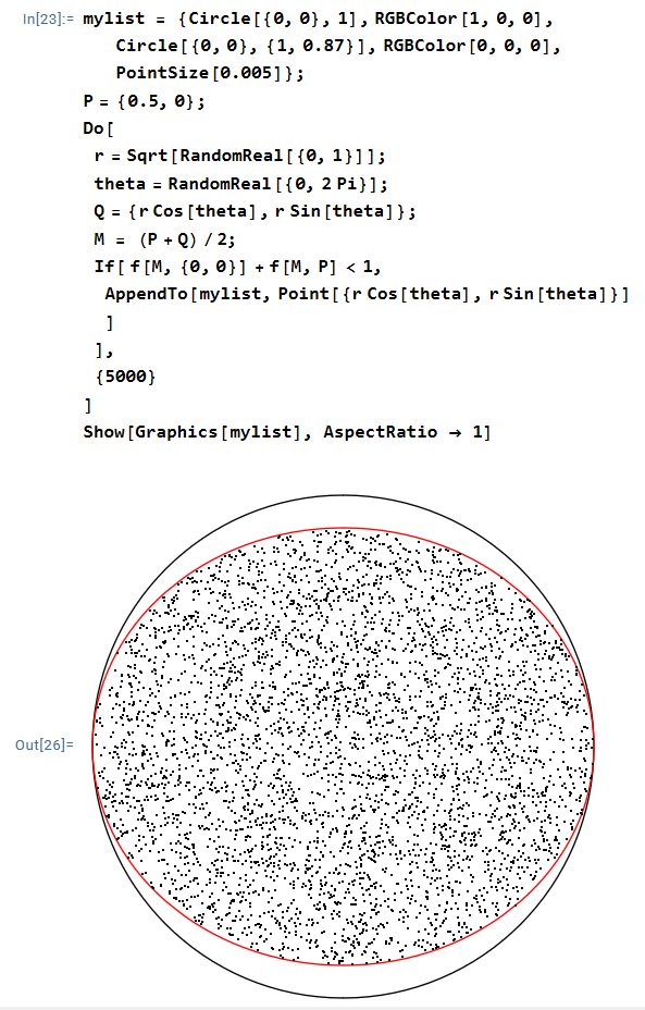
 and
and  , where the distance from the origin
  is chosen at random from
  . Unfortunately, this simple simulation generates too many points that are close to the origin and not enough that are close to the circle:
 is the same as saying that the point lies inside the circle centered at the origin with radius
  .
.![[0,1]](https://s0.wp.com/latex.php?latex=%5B0%2C1%5D&bg=ffffff&fg=000000&s=0&c=20201002) , so that
, so that  . All this to say, the above simulation did not produce points uniformly chosen from the unit circle.
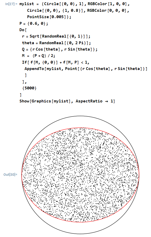
 . In other words, we will chose randomly chosen radius to have the form
  , where
  is chosen uniformly on
  ,
, 
 .
.  plus the radius of the pink circle is less than 1, or
  .
.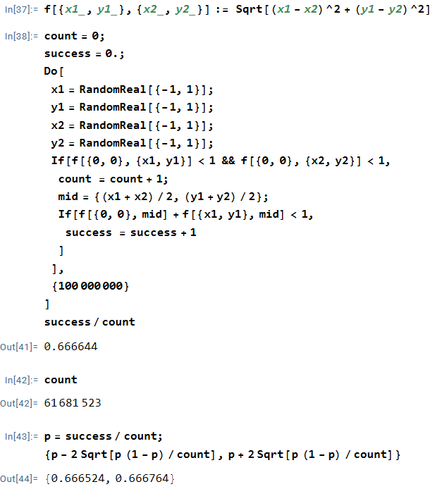
 contains
  from
from  , meaning that about
  of the simulations were simply wasted. So the only sense that this was a quick simulation was that I could type it quickly in Mathematica and then let the computer churn out a result. (I’ll talk about a better way to perform the simulation in the next post.)
 .
. and
and  and flipping the order of a double sum, I was able to show that
  .
. ,
,


![= x \displaystyle \left[ (a_0)' + \sum_{k=1}^\infty \left(a_k x^k \right)' \right]](https://s0.wp.com/latex.php?latex=%3D+x+%5Cdisplaystyle+%5Cleft%5B+%28a_0%29%27+%2B++%5Csum_%7Bk%3D1%7D%5E%5Cinfty+%5Cleft%28a_k+x%5Ek+%5Cright%29%27+%5Cright%5D&bg=ffffff&fg=000000&s=0&c=20201002)


 .
.
 and write out the full Taylor series expansion, including zero coefficients:
 ,
,


 .
. .
. ,
,

 ,
,

 .
.