

Proofs that the square root of 2 is irrational
Here’s a resource with over 25 different proofs for demonstrating that 
Mathematician maze

Approximations

An infinite number of mathematicians walk into a bar
An infinite number of mathematicians walk into a bar. The first one orders a beer, the second one orders a half a beer, the third orders a quarter of a beer, and this trend continues on for some time.
After a while, the bartender gets fed up and hands them 2 beers, shakes his head and says, “You mathematicians just don’t know your limits.”
Functions that commute
At the bottom of this post is a one-liner that I use in my classes the first time I present a theorem where two functions are permitted to commute. At many layers of the mathematics curriculum, students learn about that various functions can essentially commute with each other. In other words, the order in which the operations is performed doesn’t affect the final answer. Here’s a partial list off the top of my head:
- Arithmetic/Algebra:
. This of course is commonly called the distributive property (and not the commutative property), but the essential idea is that the same answer is obtained whether the multiplications are performed first or if the addition is performed first.
- Algebra: If
, then
.
- Algebra: If
is any real number, then
.
- Precalculus:
.
- Precalculus:
.
- Calculus: If
is continuous at an interior point
, then
.
- Calculus: If
are differentiable, then
.
- Calculus: If
.
- Calculus: If
.
- Calculus: If
.
- Calculus: If
is integrable,
.
- Calculus: For most differentiable function
.
- Probability: If
and
are random variables, then
.
- Probability: If
.
- Probability: If
.
- Probability: If
.
- Set theory: If
,
, and
are sets, then
.
- Set theory: If
.
However, there are plenty of instances when two functions do not commute. Most of these, of course, are common mistakes that students make when they first encounter these concepts. Here’s a partial list off the top of my head. (For all of these, the inequality sign means that the two sides do not have to be equal… though there may be special cases when equality happens to happen.)
- Algebra:
if
. Important special cases are
,
, and
.
- Algebra/Precalculus:
. I call this the third classic blunder.
- Precalculus:
.
- Precalculus:
,
, etc.
- Precalculus:
.
- Calculus:
.
- Calculus
- Calculus:
.
- Probability: If
.
- Probability: If
.

All this to say, it’s a big deal when two functions commute, because this doesn’t happen all the time.
 I wish I could remember the speaker’s name, but I heard the following one-liner at a state mathematics conference many years ago, and I’ve used it to great effect in my classes ever since. Whenever I present a property where two functions commute, I’ll say, “In other words, the order of operations does not matter. This is a big deal, because, in real life, the order of operations usually is important. For example, this morning, you probably got dressed and then went outside. The order was important.”
Calculators and complex numbers (Part 24)
In this series of posts, I explore properties of complex numbers that explain some surprising answers to exponential and logarithmic problems using a calculator (see video at the bottom of this post). These posts form the basis for a sequence of lectures given to my future secondary teachers.
To begin, we recall that the trigonometric form of a complex number 

where 


Theorem. If 


Definition. Let 


Definition. Let 


Technical point: for the latter two definitions, these are the principal values of the functions. In complex analysis, these are usually considered multiply-defined functions. But I’m not going to worry about this technicality here and will only consider the principal values.
This is the last post in this series, where I state some generalizations of the Laws of Exponents for complex numbers.
In yesterday’s post, we saw that 


Theorem. Let 


As we saw in a previous post, the conclusion could be incorrect outside of the above hypothesis, as 
Theorem. Let 


Theorem. Let 

Again, the conclusion of the above theorem could be incorrect outside of these hypothesis, as 

For completeness, here’s the movie that I use to engage my students when I begin this sequence of lectures.
Calculators and complex numbers (Part 23)
In this series of posts, I explore properties of complex numbers that explain some surprising answers to exponential and logarithmic problems using a calculator (see video at the bottom of this post). These posts form the basis for a sequence of lectures given to my future secondary teachers.
To begin, we recall that the trigonometric form of a complex number
where
Theorem. If
Definition. Let
Definition. Let
Technical point: for the latter two definitions, these are the principal values of the functions. In complex analysis, these are usually considered multiply-defined functions. But I’m not going to worry about this technicality here and will only consider the principal values.
In the remaining posts in this series, I want to explore which properties of exponential functions remain true when complex numbers are used.
To begin, if 


Next, one of the Laws of Exponents remains true even for complex numbers:


However, in previous posts, we’ve seen that the rules 
We can also derive the usual rules 


Next, we think like an MIT freshman and use the above Law of Exponents to observe that

Dividing, we see that
For completeness, here’s the movie that I use to engage my students when I begin this sequence of lectures.
Calculators and complex numbers (Part 22)
In this series of posts, I explore properties of complex numbers that explain some surprising answers to exponential and logarithmic problems using a calculator (see video at the bottom of this post). These posts form the basis for a sequence of lectures given to my future secondary teachers.
To begin, we recall that the trigonometric form of a complex number
where
Theorem. If
Definition. Let
At long last, we are now in position to explain the last surprising results from the calculator video below.
Definition. Suppose that
Naturally, this definition makes sense if
For example, let’s consider the computation of 

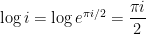
Therefore,

which is (surprisingly) a real number.
As a second example, let’s compute 

Therefore,


In other words, a problem like this is a Precalculus teacher’s dream come true, as it contains 
For completeness, here’s the movie that I use to engage my students when I begin this sequence of lectures.
Calculators and complex numbers (Part 21)
In this series of posts, I explore properties of complex numbers that explain some surprising answers to exponential and logarithmic problems using a calculator (see video at the bottom of this post). These posts form the basis for a sequence of lectures given to my future secondary teachers.
To begin, we recall that the trigonometric form of a complex number
where
Over the past few posts, we developed the following theorem for computing 
Definition. Let
Of course, this looks like what the definition ought to be if one formally applies the Laws of Logarithms to 

This is analogous to another situation when an inverse function is defined using a restricted domain, like

or

The Laws of Logarithms also may not work when nonpositive numbers are used. For example,

but

For completeness, here’s the movie that I use to engage my students when I begin this sequence of lectures.

