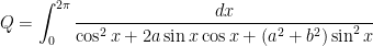
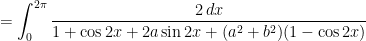
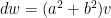
Originally, my wife had asked me to compute this integral by hand because Mathematica 4 and Mathematica 8 gave different answers. At the time, I eventually obtained the solution by multiplying the top and bottom of the integrand by

and then employing the substitution

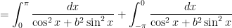
(after using trig identities to adjust the limits of integration).
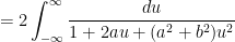
But this wasn’t the only method I tried. Indeed, I tried two or three different methods before deciding they were too messy and trying something different. So, for the rest of this series, I’d like to explore different ways that the above integral can be computed.

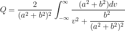
Here’s my progress so far:


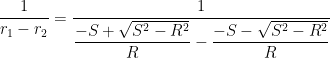
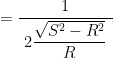
where this last integral is taken over the complex plane on the unit circle, a closed contour oriented counterclockwise. Also,
and
 ,
,
are the two distinct roots of the denominator (as long as  ). In these formulas,
 and
and 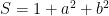 . (Also,
  is a certain angle that is now irrelevant at this point in the calculation).
This contour integral looks more complicated; however, it’s an amazing fact that integrals over closed contours can be easily evaluated by only looking at the poles of the integrand. For this integral, that means finding the values of  where the denominator is equal to 0, and then determining which of those values lie inside of the closed contour.
Let’s now see if either of the two roots of the denominator lies inside of the unit circle in the complex plane. In other words, let’s determine if  and/or
  .
.
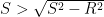
I’ll begin with  . Clearly, the numbers
  ,
,  , and
, and  are the lengths of three sides of a right triangle with hypotenuse . So, since the hypotenuse is the longest side,
or

so that
 .
.
Also, by the triangle inequality,
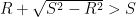


Combining these inequalities, we see that
 ,
,
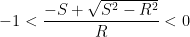
and so I see that , so that does lie inside of the contour  .
.
The second root  is easier to handle:
 .
.
Therefore, since lies outside of the contour, this root is not important for the purposes of computing the above contour integral.
Now that I’ve identified the root that lies inside of the contour, I now have to compute the residue at this root. I’ll discuss this in tomorrow’s post.

 is independent of
  , I’ll now give a fourth method.
 :
:
 Since
Since 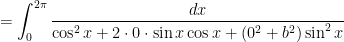


 to show that
  .
. , so that
  is a constant with respect to
  does not depend on
  ) using the Quotient Rule:
![Q'(a) = \displaystyle 2 \int_{-\infty}^{\infty} \frac{ 2a \left[ (a^2+b^2)^2 v^2 + b^2\right] - 2 (a^2+b^2) \cdot (a^2+b^2) v^2 \cdot 2a }{\left[ (a^2+b^2)^2 v^2 + b^2 \right]^2} dv](https://s0.wp.com/latex.php?latex=Q%27%28a%29+%3D+%5Cdisplaystyle+2+%5Cint_%7B-%5Cinfty%7D%5E%7B%5Cinfty%7D+%5Cfrac%7B+2a+%5Cleft%5B+%28a%5E2%2Bb%5E2%29%5E2+v%5E2+%2B+b%5E2%5Cright%5D+-+2+%28a%5E2%2Bb%5E2%29+%5Ccdot+%28a%5E2%2Bb%5E2%29+v%5E2+%5Ccdot+2a+%7D%7B%5Cleft%5B+%28a%5E2%2Bb%5E2%29%5E2+v%5E2+%2B+b%5E2+%5Cright%5D%5E2%7D+dv&bg=ffffff&fg=000000&s=0&c=20201002)
![Q'(a) = \displaystyle 4a \int_{-\infty}^{\infty} \frac{(a^2+b^2)^2 v^2 + b^2- 2 (a^2+b^2)^2 v^2}{\left[ (a^2+b^2)^2 v^2 + b^2 \right]^2} dv](https://s0.wp.com/latex.php?latex=Q%27%28a%29+%3D+%5Cdisplaystyle+4a+%5Cint_%7B-%5Cinfty%7D%5E%7B%5Cinfty%7D+%5Cfrac%7B%28a%5E2%2Bb%5E2%29%5E2+v%5E2+%2B+b%5E2-+2+%28a%5E2%2Bb%5E2%29%5E2+v%5E2%7D%7B%5Cleft%5B+%28a%5E2%2Bb%5E2%29%5E2+v%5E2+%2B+b%5E2+%5Cright%5D%5E2%7D+dv&bg=ffffff&fg=000000&s=0&c=20201002)
![Q'(a) = \displaystyle 4a \int_{-\infty}^{\infty} \frac{b^2-(a^2+b^2)^2 v^2}{\left[ (a^2+b^2)^2 v^2 + b^2 \right]^2} dv](https://s0.wp.com/latex.php?latex=Q%27%28a%29+%3D+%5Cdisplaystyle+4a+%5Cint_%7B-%5Cinfty%7D%5E%7B%5Cinfty%7D+%5Cfrac%7Bb%5E2-%28a%5E2%2Bb%5E2%29%5E2+v%5E2%7D%7B%5Cleft%5B+%28a%5E2%2Bb%5E2%29%5E2+v%5E2+%2B+b%5E2+%5Cright%5D%5E2%7D+dv&bg=ffffff&fg=000000&s=0&c=20201002)
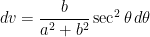
 , so that
![(a^2+b^2)^2 v^2 = (a^2+b^2)^2 \displaystyle \left[ \frac{b}{a^2+b^2} \tan \theta \right]^2 = b^2 \tan^2 \theta](https://s0.wp.com/latex.php?latex=%28a%5E2%2Bb%5E2%29%5E2+v%5E2+%3D+%28a%5E2%2Bb%5E2%29%5E2+%5Cdisplaystyle+%5Cleft%5B+%5Cfrac%7Bb%7D%7Ba%5E2%2Bb%5E2%7D+%5Ctan+%5Ctheta+%5Cright%5D%5E2+%3D+b%5E2+%5Ctan%5E2+%5Ctheta&bg=ffffff&fg=000000&s=0&c=20201002)
 to
to  , and so
![Q'(a) = \displaystyle 4a \int_{-\pi/2}^{\pi/2} \frac{b^2- b^2 \tan^2 \theta}{\left[ b^2 \tan^2 \theta + b^2 \right]^2} \frac{b}{a^2+b^2} \sec^2 \theta \, d\theta](https://s0.wp.com/latex.php?latex=Q%27%28a%29+%3D+%5Cdisplaystyle+4a+%5Cint_%7B-%5Cpi%2F2%7D%5E%7B%5Cpi%2F2%7D+%5Cfrac%7Bb%5E2-+b%5E2+%5Ctan%5E2+%5Ctheta%7D%7B%5Cleft%5B+b%5E2+%5Ctan%5E2+%5Ctheta+%2B+b%5E2+%5Cright%5D%5E2%7D+%5Cfrac%7Bb%7D%7Ba%5E2%2Bb%5E2%7D+%5Csec%5E2+%5Ctheta+%5C%2C+d%5Ctheta&bg=ffffff&fg=000000&s=0&c=20201002)
![= \displaystyle \frac{4ab^3}{a^2+b^2} \int_{-\pi/2}^{\pi/2} \frac{[1- \tan^2 \theta] \sec^2 \theta}{\left[ \tan^2 \theta +1 \right]^2} d\theta](https://s0.wp.com/latex.php?latex=%3D+%5Cdisplaystyle+%5Cfrac%7B4ab%5E3%7D%7Ba%5E2%2Bb%5E2%7D+%5Cint_%7B-%5Cpi%2F2%7D%5E%7B%5Cpi%2F2%7D+%5Cfrac%7B%5B1-+%5Ctan%5E2+%5Ctheta%5D+%5Csec%5E2+%5Ctheta%7D%7B%5Cleft%5B+%5Ctan%5E2+%5Ctheta+%2B1+%5Cright%5D%5E2%7D+d%5Ctheta&bg=ffffff&fg=000000&s=0&c=20201002)
![= \displaystyle \frac{4ab^3}{a^2+b^2} \int_{-\pi/2}^{\pi/2} \frac{[1-\tan^2 \theta] \sec^2 \theta}{\left[ \sec^2 \theta \right]^2} d\theta](https://s0.wp.com/latex.php?latex=%3D+%5Cdisplaystyle+%5Cfrac%7B4ab%5E3%7D%7Ba%5E2%2Bb%5E2%7D+%5Cint_%7B-%5Cpi%2F2%7D%5E%7B%5Cpi%2F2%7D+%5Cfrac%7B%5B1-%5Ctan%5E2+%5Ctheta%5D+%5Csec%5E2+%5Ctheta%7D%7B%5Cleft%5B+%5Csec%5E2+%5Ctheta+%5Cright%5D%5E2%7D+d%5Ctheta&bg=ffffff&fg=000000&s=0&c=20201002)
![= \displaystyle \frac{4ab^3}{a^2+b^2} \int_{-\pi/2}^{\pi/2} \frac{[1-\tan^2 \theta] \sec^2 \theta}{\sec^4 \theta} d\theta](https://s0.wp.com/latex.php?latex=%3D+%5Cdisplaystyle+%5Cfrac%7B4ab%5E3%7D%7Ba%5E2%2Bb%5E2%7D+%5Cint_%7B-%5Cpi%2F2%7D%5E%7B%5Cpi%2F2%7D+%5Cfrac%7B%5B1-%5Ctan%5E2+%5Ctheta%5D+%5Csec%5E2+%5Ctheta%7D%7B%5Csec%5E4+%5Ctheta%7D+d%5Ctheta&bg=ffffff&fg=000000&s=0&c=20201002)
![= \displaystyle \frac{4ab^3}{a^2+b^2} \int_{-\pi/2}^{\pi/2} \frac{[1- \tan^2 \theta]}{\sec^2 \theta} d\theta](https://s0.wp.com/latex.php?latex=%3D+%5Cdisplaystyle+%5Cfrac%7B4ab%5E3%7D%7Ba%5E2%2Bb%5E2%7D+%5Cint_%7B-%5Cpi%2F2%7D%5E%7B%5Cpi%2F2%7D+%5Cfrac%7B%5B1-+%5Ctan%5E2+%5Ctheta%5D%7D%7B%5Csec%5E2+%5Ctheta%7D+d%5Ctheta&bg=ffffff&fg=000000&s=0&c=20201002)
![= \displaystyle \frac{4ab^3}{a^2+b^2} \int_{-\pi/2}^{\pi/2} [1- \tan^2 \theta] \cos^2 \theta \, d\theta](https://s0.wp.com/latex.php?latex=%3D+%5Cdisplaystyle+%5Cfrac%7B4ab%5E3%7D%7Ba%5E2%2Bb%5E2%7D+%5Cint_%7B-%5Cpi%2F2%7D%5E%7B%5Cpi%2F2%7D+%5B1-+%5Ctan%5E2+%5Ctheta%5D+%5Ccos%5E2+%5Ctheta+%5C%2C+d%5Ctheta&bg=ffffff&fg=000000&s=0&c=20201002)
![= \displaystyle \frac{4ab^3}{a^2+b^2} \int_{-\pi/2}^{\pi/2} [\cos^2 \theta -\sin^2 \theta] d\theta](https://s0.wp.com/latex.php?latex=%3D+%5Cdisplaystyle+%5Cfrac%7B4ab%5E3%7D%7Ba%5E2%2Bb%5E2%7D+%5Cint_%7B-%5Cpi%2F2%7D%5E%7B%5Cpi%2F2%7D+%5B%5Ccos%5E2+%5Ctheta+-%5Csin%5E2+%5Ctheta%5D+d%5Ctheta&bg=ffffff&fg=000000&s=0&c=20201002)

![= \displaystyle \left[ \frac{2ab^3}{a^2+b^2} \sin 2\theta \right]^{\pi/2}_{-\pi/2}](https://s0.wp.com/latex.php?latex=%3D+%5Cdisplaystyle+%5Cleft%5B+%5Cfrac%7B2ab%5E3%7D%7Ba%5E2%2Bb%5E2%7D+%5Csin+2%5Ctheta+%5Cright%5D%5E%7B%5Cpi%2F2%7D_%7B-%5Cpi%2F2%7D&bg=ffffff&fg=000000&s=0&c=20201002)
![= \displaystyle \frac{2ab^3}{a^2+b^2} \left[ \sin \pi - \sin (-\pi) \right]](https://s0.wp.com/latex.php?latex=%3D+%5Cdisplaystyle+%5Cfrac%7B2ab%5E3%7D%7Ba%5E2%2Bb%5E2%7D+%5Cleft%5B+%5Csin+%5Cpi+-+%5Csin+%28-%5Cpi%29+%5Cright%5D&bg=ffffff&fg=000000&s=0&c=20201002)
![= \displaystyle \frac{2ab^3}{a^2+b^2} \left[ 0- 0 \right]](https://s0.wp.com/latex.php?latex=%3D+%5Cdisplaystyle+%5Cfrac%7B2ab%5E3%7D%7Ba%5E2%2Bb%5E2%7D+%5Cleft%5B+0-+0+%5Cright%5D&bg=ffffff&fg=000000&s=0&c=20201002)
 .
. :
:
 . Since
  , the endpoints of integration do not change, and so
 .
. without altering the value of
 .
.
 .
. and identifying the coefficient for the term
  .
. has the form
  , where
  and
and  are differentiable functions so that
  and
and  . Therefore, we may rewrite this function using the Taylor series expansion of
  about
about  :
:![f(z) = \displaystyle \frac{1}{z-r} \left[ \frac{g(z)}{h(z)} \right]](https://s0.wp.com/latex.php?latex=f%28z%29+%3D+%5Cdisplaystyle+%5Cfrac%7B1%7D%7Bz-r%7D+%5Cleft%5B+%5Cfrac%7Bg%28z%29%7D%7Bh%28z%29%7D+%5Cright%5D&bg=ffffff&fg=000000&s=0&c=20201002)
![f(z) = \displaystyle \frac{1}{z-r} \left[ a_0 + a_1 (z-r) + a_2 (z-r)^2 + a_3 (z-r)^3 + \dots \right]](https://s0.wp.com/latex.php?latex=f%28z%29+%3D+%5Cdisplaystyle+%5Cfrac%7B1%7D%7Bz-r%7D+%5Cleft%5B+a_0+%2B+a_1+%28z-r%29+%2B+a_2+%28z-r%29%5E2+%2B+a_3+%28z-r%29%5E3+%2B+%5Cdots+%5Cright%5D&bg=ffffff&fg=000000&s=0&c=20201002)

![\displaystyle \lim_{z \to r} (z-r) f(z) = \displaystyle \lim_{z \to r} \left[ a_0 + a_1 (z-r) + a_2 (z-r)^2 + a_3 (z-r)^3 + \dots \right] = a_0](https://s0.wp.com/latex.php?latex=%5Cdisplaystyle+%5Clim_%7Bz+%5Cto+r%7D+%28z-r%29+f%28z%29+%3D+%5Cdisplaystyle+%5Clim_%7Bz+%5Cto+r%7D+%5Cleft%5B+a_0+%2B+a_1+%28z-r%29+%2B+a_2+%28z-r%29%5E2+%2B+a_3+%28z-r%29%5E3+%2B+%5Cdots+%5Cright%5D+%3D+a_0&bg=ffffff&fg=000000&s=0&c=20201002)
 . Notice that
 ,
, is the original denominator of
 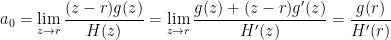 .
. and
and  , so that
  . Therefore, the residue at

 ,
, , or the constant term in the Taylor expansion of
 . Therefore, the residue at
  , matching the result found earlier.
 times the sum of the residues within the contour; see


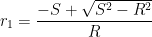
![S^2 - R^2 = [(1 + a^2 + b^2) + (1-a^2-b^2)][(1 + a^2 + b^2) - (1 - a^2 -b^2)] - 4a^2](https://s0.wp.com/latex.php?latex=S%5E2+-+R%5E2+%3D+%5B%281+%2B+a%5E2+%2B+b%5E2%29+%2B+%281-a%5E2-b%5E2%29%5D%5B%281+%2B+a%5E2+%2B+b%5E2%29+-+%281+-+a%5E2+-b%5E2%29%5D+-+4a%5E2&bg=ffffff&fg=000000&s=0&c=20201002)
![S^2 - R^2 = 2[2 a^2 + 2b^2] - 4a^2](https://s0.wp.com/latex.php?latex=S%5E2+-+R%5E2+%3D+2%5B2+a%5E2+%2B+2b%5E2%5D+-+4a%5E2&bg=ffffff&fg=000000&s=0&c=20201002)


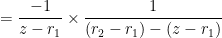

![= \displaystyle \frac{-1}{z-r_1} \times \frac{1}{r_2-r_1} \left[ 1 + \left( \displaystyle \frac{z-r_1}{r_2-r_1} \right) + \left( \displaystyle \frac{z-r_1}{r_2-r_1} \right)^2 + \left( \displaystyle \frac{z-r_1}{r_2-r_1} \right)^3 + \dots \right]](https://s0.wp.com/latex.php?latex=%3D+%5Cdisplaystyle+%5Cfrac%7B-1%7D%7Bz-r_1%7D+%5Ctimes+%5Cfrac%7B1%7D%7Br_2-r_1%7D+%5Cleft%5B+1+%2B+%5Cleft%28+%5Cdisplaystyle+%5Cfrac%7Bz-r_1%7D%7Br_2-r_1%7D+%5Cright%29+%2B+%5Cleft%28+%5Cdisplaystyle+%5Cfrac%7Bz-r_1%7D%7Br_2-r_1%7D+%5Cright%29%5E2+%2B+%5Cleft%28+%5Cdisplaystyle+%5Cfrac%7Bz-r_1%7D%7Br_2-r_1%7D+%5Cright%29%5E3+%2B+%5Cdots+%5Cright%5D&bg=ffffff&fg=000000&s=0&c=20201002)

 term in the above series. Therefore,
 is
is 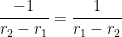


 .
. as long as
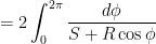
  to evaluate this last integral. Now, I’ll instead use contour integration; see
  ,
,![\cos \phi = \displaystyle \frac{1}{2} \left[z + \displaystyle \frac{1}{z} \right]](https://s0.wp.com/latex.php?latex=%5Ccos+%5Cphi+%3D+%5Cdisplaystyle+%5Cfrac%7B1%7D%7B2%7D+%5Cleft%5Bz+%2B+%5Cdisplaystyle+%5Cfrac%7B1%7D%7Bz%7D+%5Cright%5D&bg=ffffff&fg=000000&s=0&c=20201002)

 to a the unit circle
 ![Q = 2 \displaystyle \oint_C \frac{\displaystyle -\frac{i}{z} dz}{S + \displaystyle \frac{R}{2} \left[z + \displaystyle \frac{1}{z} \right]}](https://s0.wp.com/latex.php?latex=Q+%3D+2+%5Cdisplaystyle+%5Coint_C+%5Cfrac%7B%5Cdisplaystyle+-%5Cfrac%7Bi%7D%7Bz%7D+dz%7D%7BS+%2B+%5Cdisplaystyle+%5Cfrac%7BR%7D%7B2%7D+%5Cleft%5Bz+%2B+%5Cdisplaystyle+%5Cfrac%7B1%7D%7Bz%7D+%5Cright%5D%7D&bg=ffffff&fg=000000&s=0&c=20201002)

