In my capstone class for future secondary math teachers, I ask my students to come up with ideas for engaging their students with different topics in the secondary mathematics curriculum. In other words, the point of the assignment was not to devise a full-blown lesson plan on this topic. Instead, I asked my students to think about three different ways of getting their students interested in the topic in the first place.
I plan to share some of the best of these ideas on this blog (after asking my students’ permission, of course).
This student submission comes from my former student Michelle McKay. Her topic, from Probability: Venn diagrams.

A. What interesting word problems using this topic can your students do now?
In my opinion, you can create a word problem with Venn diagrams on just about anything. To make a word problem more interesting, you can relate the problem to an upcoming event or holiday, make a cultural reference, or even discuss students’ hobbies (i.e. video games, books, etc.).
On Valentine’s Day, a survey of what gifts a women received from their significant other yielded surprising results.
76% of the women surveyed received a card.
72% received chocolate.
49% received flowers.
21% received chocolate and a card.
5% received a card and flowers.
7% received chocolate and flowers.
33% received chocolate, a card, and flowers.
If a woman from the survey was selected at random, what would the probability of her having not received a Valentine’s Day gift be? What is the probability that she received any combination of two gifts? What is the probability that she received a card and flowers, but not chocolate?
B. How can this topic be used in your students’ future courses in mathematics or science?
Venn diagrams are an excellent way to organize information. They can organize and be a visual representation of gathered statistics (like in the above section). They can also organize general ideas and concepts, distinguishing them as unique or shared amongst other ideas/concepts. A student can use Venn diagrams in either of these manners for both math and science classes of any difficulty.
B. How does this topic extend what your students should have learned in previous courses?
When using Venn diagrams to represent statistics, it reinforces the idea that parts cannot be larger than the whole. We know when using Venn diagrams for statistical data that the decimals must add up to 1 to represent 100%. Students should realize that adding the decimals and getting a number that is larger than or smaller than 1 means they miscalculated or there is “missing” data. By “missing” data, I mean to say that they did not enter in all the given information correctly.

 chance in
  . What is the probability that, after playing
  . Therefore, the chance of not winning
  , which we can approximate with a calculator.
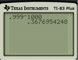

 ? Then the probability would be
  .
.
 , so that the probability of never winning for both problems is approximately
  .
.
 , we find
 , we have
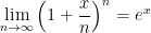
![\ln \left[ \displaystyle \lim_{n \to \infty} \left(1 + \frac{x}{n}\right)^n \right] = \displaystyle \lim_{n \to \infty} \ln \left[ \left(1 + \frac{x}{n}\right)^n \right]](https://s0.wp.com/latex.php?latex=%5Cln+%5Cleft%5B+%5Cdisplaystyle+%5Clim_%7Bn+%5Cto+%5Cinfty%7D+%5Cleft%281+%2B+%5Cfrac%7Bx%7D%7Bn%7D%5Cright%29%5En+%5Cright%5D+%3D+%5Cdisplaystyle+%5Clim_%7Bn+%5Cto+%5Cinfty%7D+%5Cln+%5Cleft%5B+%5Cleft%281+%2B+%5Cfrac%7Bx%7D%7Bn%7D%5Cright%29%5En+%5Cright%5D&bg=ffffff&fg=000000&s=0&c=20201002)
![\ln \left[ \displaystyle \lim_{n \to \infty} \left(1 + \frac{x}{n}\right)^n \right] = \displaystyle \lim_{n \to \infty} n \ln \left(1 + \frac{x}{n}\right)](https://s0.wp.com/latex.php?latex=%5Cln+%5Cleft%5B+%5Cdisplaystyle+%5Clim_%7Bn+%5Cto+%5Cinfty%7D+%5Cleft%281+%2B+%5Cfrac%7Bx%7D%7Bn%7D%5Cright%29%5En+%5Cright%5D+%3D+%5Cdisplaystyle+%5Clim_%7Bn+%5Cto+%5Cinfty%7D+n+%5Cln+%5Cleft%281+%2B+%5Cfrac%7Bx%7D%7Bn%7D%5Cright%29&bg=ffffff&fg=000000&s=0&c=20201002)
![\ln \left[ \displaystyle \lim_{n \to \infty} \left(1 + \frac{x}{n}\right)^n \right] = \displaystyle \lim_{n \to \infty} \frac{ \displaystyle \ln \left(1 + \frac{x}{n}\right)}{\displaystyle \frac{1}{n}}](https://s0.wp.com/latex.php?latex=%5Cln+%5Cleft%5B+%5Cdisplaystyle+%5Clim_%7Bn+%5Cto+%5Cinfty%7D+%5Cleft%281+%2B+%5Cfrac%7Bx%7D%7Bn%7D%5Cright%29%5En+%5Cright%5D+%3D+%5Cdisplaystyle+%5Clim_%7Bn+%5Cto+%5Cinfty%7D+%5Cfrac%7B+%5Cdisplaystyle+%5Cln+%5Cleft%281+%2B+%5Cfrac%7Bx%7D%7Bn%7D%5Cright%29%7D%7B%5Cdisplaystyle+%5Cfrac%7B1%7D%7Bn%7D%7D&bg=ffffff&fg=000000&s=0&c=20201002)
 as
as  , and so we may use L’Hopital’s rule, differentiating both the numerator and the denominator with respect to
  .
.![\ln \left[ \displaystyle \lim_{n \to \infty} \left(1 + \frac{x}{n}\right)^n \right] = \displaystyle \lim_{n \to \infty} \frac{ \displaystyle \frac{1}{1 + \frac{x}{n}} \cdot \frac{-x}{n^2} }{\displaystyle \frac{-1}{n^2}}](https://s0.wp.com/latex.php?latex=%5Cln+%5Cleft%5B+%5Cdisplaystyle+%5Clim_%7Bn+%5Cto+%5Cinfty%7D+%5Cleft%281+%2B+%5Cfrac%7Bx%7D%7Bn%7D%5Cright%29%5En+%5Cright%5D+%3D+%5Cdisplaystyle+%5Clim_%7Bn+%5Cto+%5Cinfty%7D+%5Cfrac%7B+%5Cdisplaystyle+%5Cfrac%7B1%7D%7B1+%2B+%5Cfrac%7Bx%7D%7Bn%7D%7D+%5Ccdot+%5Cfrac%7B-x%7D%7Bn%5E2%7D+%7D%7B%5Cdisplaystyle+%5Cfrac%7B-1%7D%7Bn%5E2%7D%7D&bg=ffffff&fg=000000&s=0&c=20201002)
![\ln \left[ \displaystyle \lim_{n \to \infty} \left(1 + \frac{x}{n}\right)^n \right] = \displaystyle \lim_{n \to \infty} \displaystyle \frac{x}{1 + \frac{x}{n}}](https://s0.wp.com/latex.php?latex=%5Cln+%5Cleft%5B+%5Cdisplaystyle+%5Clim_%7Bn+%5Cto+%5Cinfty%7D+%5Cleft%281+%2B+%5Cfrac%7Bx%7D%7Bn%7D%5Cright%29%5En+%5Cright%5D+%3D+%5Cdisplaystyle+%5Clim_%7Bn+%5Cto+%5Cinfty%7D+%5Cdisplaystyle+%5Cfrac%7Bx%7D%7B1+%2B+%5Cfrac%7Bx%7D%7Bn%7D%7D&bg=ffffff&fg=000000&s=0&c=20201002)
![\ln \left[ \displaystyle \lim_{n \to \infty} \left(1 + \frac{x}{n}\right)^n \right] = \displaystyle \frac{x}{1 + 0}](https://s0.wp.com/latex.php?latex=%5Cln+%5Cleft%5B+%5Cdisplaystyle+%5Clim_%7Bn+%5Cto+%5Cinfty%7D+%5Cleft%281+%2B+%5Cfrac%7Bx%7D%7Bn%7D%5Cright%29%5En+%5Cright%5D+%3D+%5Cdisplaystyle+%5Cfrac%7Bx%7D%7B1+%2B+0%7D&bg=ffffff&fg=000000&s=0&c=20201002)
![\ln \left[ \displaystyle \lim_{n \to \infty} \left(1 + \frac{x}{n}\right)^n \right] = x](https://s0.wp.com/latex.php?latex=%5Cln+%5Cleft%5B+%5Cdisplaystyle+%5Clim_%7Bn+%5Cto+%5Cinfty%7D+%5Cleft%281+%2B+%5Cfrac%7Bx%7D%7Bn%7D%5Cright%29%5En+%5Cright%5D+%3D+x&bg=ffffff&fg=000000&s=0&c=20201002)

 can be derived from the formula for discrete compound interest
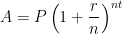
 , when


 . See
. See  actually converges and must correspond to a real number. See
  must have a repeating block of length
  which contains the digits of
  . See
. See