Polynomial Long Division and Megan Moroney

A brief clip from Megan Moroney’s video “I’m Not Pretty” correctly uses polynomial long division to establish that $2x+3$ is a factor of $2x^4+5x^3+7x^2+16x+15$ . Even more amazingly, the fact that the remainder is $0$ actually fits artistically with the video.

And while I have her music on my mind, I can’t resist sharing her masterpiece “Tennessee Orange” and its playful commentary on the passion of college football fans.

Lagrange Points and Polynomial Equations: Index

I’m doing something that I should have done a long time ago: collecting a series of posts into one single post. The links below show my series on Lagrange points.

Part 1: Introduction

Part 2: Finding $L_1$

Part 3: Finding $L_2$

Part 4: A more analytical way of finding $L_1$ and $L_2$

Part 5: Historical anecdote: Lagrange made a careless mistake!

Solving Problems Submitted to MAA Journals (Part 6d)

The following problem appeared in Volume 97, Issue 3 (2024) of Mathematics Magazine.

Two points $P$ and $Q$ are chosen at random (uniformly) from the interior of a unit circle. What is the probability that the circle whose diameter is segment $overline{PQ}$ lies entirely in the interior of the unit circle?

As discussed in a previous post, I guessed from simulation that the answer is $2/3$ . Naturally, simulation is not a proof, and so I started thinking about how to prove this.

My first thought was to make the problem simpler by letting only one point be chosen at random instead of two. Suppose that the point $P$ is fixed at a distance $t$ from the origin. What is the probability that the point $Q$ , chosen at random, uniformly, from the interior of the unit circle, has the desired property?

My second thought is that, by radial symmetry, I could rotate the figure so that the point $P$ is located at $(t,0)$ . In this way, the probability in question is ultimately going to be a function of $t$ .

There is a very nice way to compute such probabilities since $Q$ is chosen at uniformly from the unit circle. Let $A_t$ be the set of all points $Q$ within the unit circle that have the desired property. Since the area of the unit circle is $\pi(1)^2 = \pi$ , the probability of desired property happening is

$\displaystyle \frac{\hbox{area}(A_t)}{\pi}$ .

Based on the simulations discussed in the previous post, my guess was that $A_t$ was the interior of an ellipse centered at the origin with a semimajor axis of length $1$ and a semiminor axis of length $\sqrt{1-t^2}$ . Now I had to think about how to prove this.

As noted earlier in this series, the circle with diameter $\overline{PQ}$ will lie within the unit circle exactly when $MO+MP < 1$ , where $M$ is the midpoint of $\overline{PQ}$ . So suppose that $P$ has coordinates $(t,0)$ , where $t$ is known, and let the coordinates of $Q$ be $(x,y)$ . Then the coordinates of $M$ will be

$\displaystyle \left( \frac{x+t}{2}, \frac{y}{2} \right)$ ,

so that

$MO = \displaystyle \sqrt{ \left( \frac{x+t}{2} \right)^2 + \left( \frac{y}{2} \right)^2}$

and

$MP = \displaystyle \sqrt{ \left( \frac{x+t}{2} - t\right)^2 + \left( \frac{y}{2} \right)^2} = \sqrt{ \left( \frac{x-t}{2} \right)^2 + \left( \frac{y}{2} \right)^2}$ .

Therefore, the condition $MO+MP < 1$ (again, equivalent to the condition that the circle with diameter $\overline{PQ}$ lies within the unit circle) becomes

$\displaystyle \sqrt{ \left( \frac{x+t}{2} \right)^2 + \left( \frac{y}{2} \right)^2} + \sqrt{ \left( \frac{x-t}{2} \right)^2 + \left( \frac{y}{2} \right)^2} < 1$ ,

which simplifies to

$\displaystyle \sqrt{ \frac{1}{4} \left[ (x+t)^2 + y^2 \right]} + \sqrt{ \frac{1}{4} \left[ (x-t)^2 + y^2 \right]} < 1$

$\displaystyle \frac{1}{2}\sqrt{ (x+t)^2 + y^2} + \frac{1}{2}\sqrt{ (x-t)^2 + y^2} < 1$

$\displaystyle \sqrt{ (x+t)^2 + y^2} + \sqrt{ (x-t)^2 + y^2} < 2$ .

When I saw this, light finally dawned. Given two points $F_1$ and $F_2$ , called the foci, an ellipse is defined to be the set of all points $Q$ so that $QF_1 + QF_2 = 2a$ , where $a$ is a constant. If the coordinates of $Q$ , $F_1$ , and $F_2$ are $(x,y)$ , $(c,0)$ , and $(-c,0)$ , then this becomes

$\displaystyle \sqrt{ (x+c)^2 + y^2} + \sqrt{ (x-c)^2 + y^2} = 2a$ .

Therefore, the set $A_t$ is the interior of an ellipse centered at the origin with $a = 1$ and $c = t$ . Furthermore, $a = 1$ is the semimajor axis of the ellipse, while the semiminor axis is equal to $b = \sqrt{a^2-c^2} = \sqrt{1-t^2}$ .

At last, I could now return to the original question. Suppose that the point $P$ is fixed at a distance $t$ from the origin. What is the probability that the point $Q$ , chosen at random, uniformly, from the interior of the unit circle, has the property that the circle with diameter $\overline{PQ}$ lies within the unit circle? Since $A_t$ is a subset of the interior of the unit circle, we see that this probability is equal to

$\displaystyle \frac{\hbox{area}(A_t)}{\hbox{area of unit circle}} = \frac{\pi \cdot 1 \cdot \sqrt{1-t^2}}{\pi (1)^2} = \sqrt{1-t^2}$ .

In the next post, I’ll use this intermediate step to solve the original question.

Solving Problems Submitted to MAA Journals (Part 5e)

The following problem appeared in Volume 96, Issue 3 (2023) of Mathematics Magazine.

Evaluate the following sums in closed form:

$f(x) = \displaystyle \sum_{n=0}^\infty \left( \cos x - 1 + \frac{x^2}{2!} - \frac{x^4}{4!} \dots + (-1)^{n-1} \frac{x^{2n}}{(2n)!} \right)$

and

$g(x) = \displaystyle \sum_{n=0}^\infty \left( \sin x - x + \frac{x^3}{3!} - \frac{x^5}{5!} \dots + (-1)^{n-1} \frac{x^{2n+1}}{(2n+1)!} \right)$ .

By using the Taylor series expansions of $\sin x$ and $\cos x$ and flipping the order of a double sum, I was able to show that

$f(x) = -\displaystyle \frac{x \sin x}{2} \qquad \hbox{and} \qquad g(x) = \frac{x\cos x - \sin x}{2}$ .

I immediately got to thinking: there’s nothing particularly special about $\sin x$ and $\cos x$ for this analysis. Is there a way of generalizing this result to all functions with a Taylor series expansion?

Suppose

$h(x) = \displaystyle \sum_{k=0}^\infty a_k x^k$ ,

and let’s use the same technique to evaluate

$\displaystyle \sum_{n=0}^\infty \left( h(x) - \sum_{k=0}^n a_k x^k \right) = \sum_{n=0}^\infty \sum_{k=n+1}^\infty a_k x^k$

$= \displaystyle \sum_{k=1}^\infty \sum_{n=0}^{k-1} a_k x^k$

$= \displaystyle \sum_{k=1}^\infty k a_k x^k$

$= x \displaystyle \sum_{k=1}^\infty k a_k x^{k-1}$

$= x \displaystyle \sum_{k=1}^\infty \left(a_k x^k \right)'$

$= x \displaystyle \left[ (a_0)' + \sum_{k=1}^\infty \left(a_k x^k \right)' \right]$

$= x \displaystyle \sum_{k=0}^\infty \left(a_k x^k \right)'$

$= x \displaystyle \left( \sum_{k=0}^\infty a_k x^k \right)'$

$= x h'(x)$ .

To see why this matches our above results, let’s start with $h(x) = \cos x$ and write out the full Taylor series expansion, including zero coefficients:

$\cos x = 1 + 0x - \displaystyle \frac{x^2}{2!} + 0x^3 + \frac{x^4}{4!} + 0x^5 - \frac{x^6}{6!} \dots$ ,

so that

$x (\cos x)' = \displaystyle \sum_{n=0}^\infty \left( \cos x - \sum_{k=0}^n a_k x^k \right)$

$-x \sin x= \displaystyle \left(\cos x - 1 \right) + \left(\cos x - 1 + 0x \right) + \left( \cos x -1 + 0x + \frac{x^2}{2!} \right) + \left( \cos x -1 + 0x + \frac{x^2}{2!} + 0x^3 \right)$

$\displaystyle + \left( \cos x -1 + 0x + \frac{x^2}{2!} + 0x^3 - \frac{x^4}{4!} \right) + \left( \cos x -1 + 0x + \frac{x^2}{2!} + 0x^3 - \frac{x^4}{4!} + 0x^5 \right) \dots$

After dropping the zero terms and collecting, we obtain

$-x \sin x= \displaystyle 2 \left(\cos x - 1 \right) + 2 \left( \cos x -1 + \frac{x^2}{2!} \right) + 2 \left( \cos x -1 + \frac{x^2}{2!} - \frac{x^4}{4!} \right) \dots$

$-x \sin x = 2 f(x)$

$\displaystyle -\frac{x \sin x}{2} = f(x)$ .

A similar calculation would apply to any even function $h(x)$ .

We repeat for

$h(x) = \sin x = 0 + x + 0x^2 - \displaystyle \frac{x^3}{3!} + 0x^4 + \frac{x^5}{5!} + 0x^6 - \frac{x^7}{7!} \dots$ ,

so that

$x (\sin x)' = (\sin x - 0) + (\sin x - 0 - x) + (\sin x - 0 - x + 0x^2)$

$+ \displaystyle \left( \sin x - 0 - x + 0x^2 + \frac{x^3}{3!} \right) + \left( \sin x - 0 - x + 0x^2 + \frac{x^3}{3!} + 0x^4 \right)$

$+ \displaystyle \left( \sin x - 0 - x + 0x^2 + \frac{x^3}{3!} + 0x^4 - \frac{x^5}{5!} \right) + \left( \sin x - 0 - x + 0x^2 + \frac{x^3}{3!} + 0x^4 - \frac{x^5}{5!} + 0 x^6 \right) \dots$ ,

$x\cos x - \sin x = 2(\sin x - x) + \displaystyle 2\left(\sin x - x + \frac{x^3}{3!} \right) + 2 \left( \sin x - x + \frac{x^3}{3!} - \frac{x^5}{5!} \right) \dots$

$x \cos x - \sin x = 2 g(x)$

$\displaystyle \frac{x \cos x - \sin x}{2} = g(x)$ .

A similar argument applies for any odd function $h(x)$ .

Solving Problems Submitted to MAA Journals (Part 5c)

The following problem appeared in Volume 96, Issue 3 (2023) of Mathematics Magazine.

Evaluate the following sums in closed form:

$f(x) = \displaystyle \sum_{n=0}^\infty \left( \cos x - 1 + \frac{x^2}{2!} - \frac{x^4}{4!} \dots + (-1)^{n-1} \frac{x^{2n}}{(2n)!} \right)$

and

$g(x) = \displaystyle \sum_{n=0}^\infty \left( \sin x - x + \frac{x^3}{3!} - \frac{x^5}{5!} \dots + (-1)^{n-1} \frac{x^{2n+1}}{(2n+1)!} \right)$ .

In the previous post, we showed that $f(x) = - \frac{1}{2} x \sin x$ by writing the series as a double sum and then reversing the order of summation. We proceed with very similar logic to evaluate $g(x)$ . Since

$\sin x = \displaystyle \sum_{k=0}^\infty (-1)^k \frac{x^{2k+1}}{(2k+1)!}$

is the Taylor series expansion of $\sin x$ , we may write $g(x)$ as

$g(x) = \displaystyle \sum_{n=0}^\infty \left( \sum_{k=0}^\infty (-1)^k \frac{x^{2k+1}}{(2k+1)!} - \sum_{k=0}^n (-1)^k \frac{x^{2k+1}}{(2k+1)!} \right)$

$= \displaystyle \sum_{n=0}^\infty \sum_{k=n+1}^\infty (-1)^k \frac{x^{2k+1}}{(2k+1)!}$

As before, we employ one of my favorite techniques from the bag of tricks: reversing the order of summation. Also as before, the inner sum is inner sum is independent of $n$ , and so the inner sum is simply equal to the summand times the number of terms. We see that

$g(x) = \displaystyle \sum_{k=1}^\infty \sum_{n=0}^{k-1} (-1)^k \frac{x^{2k+1}}{(2k+1)!}$

$= \displaystyle \sum_{k=1}^\infty (-1)^k \cdot k \frac{x^{2k+1}}{(2k+1)!}$

$= \displaystyle \frac{1}{2} \sum_{k=1}^\infty (-1)^k \cdot 2k \frac{x^{2k+1}}{(2k+1)!}$ .

At this point, the solution for $g(x)$ diverges from the previous solution for $f(x)$ . I want to cancel the factor of $2k$ in the summand; however, the denominator is

$(2k+1)! = (2k+1)(2k)!$ ,

and $2k$ doesn’t cancel cleanly with $(2k+1)$ . Hypothetically, I could cancel as follows:

$\displaystyle \frac{2k}{(2k+1)!} = \frac{2k}{(2k+1)(2k)(2k-1)!} = \frac{1}{(2k+1)(2k-1)!}$ ,

but that introduces an extra $(2k+1)$ in the denominator that I’d rather avoid.

So, instead, I’ll write $2k$ as $(2k+1)-1$ and then distribute and split into two different sums:

$g(x) = \displaystyle \frac{1}{2} \sum_{k=1}^\infty (-1)^k \cdot 2k \frac{x^{2k+1}}{(2k+1)!}$

$= \displaystyle \frac{1}{2} \sum_{k=1}^\infty (-1)^k (2k+1-1) \frac{x^{2k+1}}{(2k+1)!}$

$= \displaystyle \frac{1}{2} \sum_{k=1}^\infty \left[ (-1)^k (2k+1) \frac{x^{2k+1}}{(2k+1)!} - (-1)^k \cdot 1 \frac{x^{2k+1}}{(2k+1)!} \right]$

$= \displaystyle \frac{1}{2} \sum_{k=1}^\infty (-1)^k (2k+1) \frac{x^{2k+1}}{(2k+1)!} - \frac{1}{2} \sum_{k=1}^\infty (-1)^k \frac{x^{2k+1}}{(2k+1)!}$

$= \displaystyle \frac{1}{2} \sum_{k=1}^\infty (-1)^k (2k+1) \frac{x^{2k+1}}{(2k+1)(2k)!} - \frac{1}{2} \sum_{k=1}^\infty (-1)^k \frac{x^{2k+1}}{(2k+1)!}$

$= \displaystyle \frac{1}{2} \sum_{k=1}^\infty (-1)^k \frac{x^{2k+1}}{(2k)!} - \frac{1}{2} \sum_{k=1}^\infty (-1)^k \frac{x^{2k+1}}{(2k+1)!}$ .

At this point, I factored out a power of $x$ from the first sum. In this way, the two sums are the Taylor series expansions of $\cos x$ and $\sin x$ :

$g(x) = \displaystyle \frac{x}{2} \sum_{k=1}^\infty (-1)^k \cdot \frac{x^{2k}}{(2k)!} - \frac{1}{2} \sum_{k=1}^\infty (-1)^k \frac{x^{2k+1}}{(2k+1)!}$

$= \displaystyle \frac{x}{2} \cos x - \frac{1}{2} \sin x$

$= \displaystyle \frac{x \cos x - \sin x}{2}$ .

This was sufficiently complicated that I was unable to guess this solution by experimenting with Mathematica; nevertheless, Mathematica can give graphical confirmation of the solution since the graphs of the two expressions overlap perfectly.

Solving Problems Submitted to MAA Journals (Part 5b)

The following problem appeared in Volume 96, Issue 3 (2023) of Mathematics Magazine.

Evaluate the following sums in closed form:

$f(x) = \displaystyle \sum_{n=0}^\infty \left( \cos x - 1 + \frac{x^2}{2!} - \frac{x^4}{4!} \dots + (-1)^{n-1} \frac{x^{2n}}{(2n)!} \right)$

and

$g(x) = \displaystyle \sum_{n=0}^\infty \left( \sin x - x + \frac{x^3}{3!} - \frac{x^5}{5!} \dots + (-1)^{n-1} \frac{x^{2n+1}}{(2n+1)!} \right)$ .

We start with $f(x)$ and the Taylor series

$\cos x = \displaystyle \sum_{k=0}^\infty (-1)^k \frac{x^{2k}}{(2k)!}$ .

With this, $f(x)$ can be written as

$f(x) = \displaystyle \sum_{n=0}^\infty \left( \sum_{k=0}^\infty (-1)^k \frac{x^{2k}}{(2k)!} - \sum_{k=0}^n (-1)^k \frac{x^{2k}}{(2k)!} \right)$

$= \displaystyle \sum_{n=0}^\infty \sum_{k=n+1}^\infty (-1)^k \frac{x^{2k}}{(2k)!}$ .

At this point, my immediate thought was one of my favorite techniques from the bag of tricks: reversing the order of summation. (Two or three chapters of my Ph.D. theses derived from knowing when to apply this technique.) We see that

$f(x) = \displaystyle \sum_{k=1}^\infty \sum_{n=0}^{k-1} (-1)^k \frac{x^{2k}}{(2k)!}$ .

At this point, the inner sum is independent of $n$ , and so the inner sum is simply equal to the summand times the number of terms. Since there are $k$ terms for the inner sum ( $n = 0, 1, \dots, k-1$ ), we see

$f(x) = \displaystyle \sum_{k=1}^\infty (-1)^k \cdot k \frac{x^{2k}}{(2k)!}$ .

To simplify, we multiply top and bottom by 2 so that the first term of $(2k)!$ cancels:

$f(x) = \displaystyle \frac{1}{2} \sum_{k=1}^\infty (-1)^k \cdot 2k \frac{x^{2k}}{(2k)(2k-1)!}$

$= \displaystyle \frac{1}{2} \sum_{k=1}^\infty (-1)^k \frac{x^{2k}}{(2k-1)!}$

At this point, I factored out a $(-1)$ and a power of $x$ to make the sum match the Taylor series for $\sin x$ :

$f(x) = \displaystyle -\frac{x}{2} \sum_{k=1}^\infty (-1)^{k-1} \frac{x^{2k-1}}{(2k-1)!} = -\frac{x \sin x}{2}$ .

I was unsurprised but comforted that this matched the guess I had made by experimenting with Mathematica.

Solving Problems Submitted to MAA Journals (Part 5a)

The following problem appeared in Volume 96, Issue 3 (2023) of Mathematics Magazine.

Evaluate the following sums in closed form:

$\displaystyle \sum_{n=0}^\infty \left( \cos x - 1 + \frac{x^2}{2!} - \frac{x^4}{4!} \dots + (-1)^{n-1} \frac{x^{2n}}{(2n)!} \right)$

and

$\displaystyle \sum_{n=0}^\infty \left( \sin x - x + \frac{x^3}{3!} - \frac{x^5}{5!} \dots + (-1)^{n-1} \frac{x^{2n+1}}{(2n+1)!} \right)$ .

When I first read this problem, I immediately noticed that

$\displaystyle 1 - \frac{x^2}{2!} + \frac{x^4}{4!} \dots - (-1)^{n-1} \frac{x^{2n}}{(2n)!} \right)$

is a Taylor polynomial of $\cos x$ and

$\displaystyle x - \frac{x^3}{3!} + \frac{x^5}{5!} \dots - (-1)^{n-1} \frac{x^{2n+1}}{(2n+1)!} \right)$

is a Taylor polynomial of $\sin x$ . In other words, the given expressions are the sums of the tail-sums of the Taylor series for $\cos x$ and $\sin x$ .

As usual when stumped, I used technology to guide me. Here’s the graph of the first sum, adding the first 50 terms.

I immediately notice that the function oscillates, which makes me suspect that the answer involves either $\cos x$ or $\sin x$ . I also notice that the sizes of oscillations increase as $|x|$ increases, so that the answer should have the form $g(x) \cos x$ or $g(x) \sin x$ , where $g$ is an increasing function. I also notice that the graph is symmetric about the origin, so that the function is even. I also notice that the graph passes through the origin.

So, taking all of that in, one of my first guesses was $y = x \sin x$ , which is satisfies all of the above criteria.

That’s not it, but it’s not far off. The oscillations of my guess in orange are too big and they’re inverted from the actual graph in blue. After some guessing, I eventually landed on $y = -\frac{1}{2} x \sin x$ .

That was a very good sign… the two graphs were pretty much on top of each other. That’s not a proof that $-\frac{1}{2} x \sin x$ is the answer, of course, but it’s certainly a good indicator.

I didn’t have the same luck with the other sum; I could graph it but wasn’t able to just guess what the curve could be.

Solving Problems Submitted to MAA Journals (Part 3)

The following problem appeared in Volume 53, Issue 4 (2022) of The College Mathematics Journal.

Define, for every non-negative integer $n$ , the $n$ th Catalan number by

$C_n := \displaystyle \frac{1}{n+1} {2n \choose n}$ .

Consider the sequence of complex polynomials in $z$ defined by $z_k := z_{k-1}^2 + z$ for every non-negative integer $k$ , where $z_0 := z$ . It is clear that $z_k$ has degree $2^k$ and thus has the representation

$z_k =\displaystyle \sum_{n=1}^{2^k} M_{n,k} z^n$ ,

where each $M_{n,k}$ is a positive integer. Prove that $M_{n,k} = C_{n-1}$ for $1 \le n \le k+1$ .

This problem appeared in the same issue as the probability problem considered in the previous two posts. Looking back, I think that the confidence that I gained by solving that problem gave me the persistence to solve this problem as well.

My first thought when reading this problem was something like “This involves sums, polynomials, and binomial coefficients. And since the sequence is recursively defined, it’s probably going to involve a proof by mathematical induction. I can do this.”

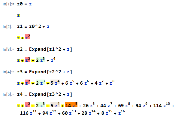
My second thought was to use Mathematica to develop my own intuition and to confirm that the claimed pattern actually worked for the first few values of $z_k$ .

As claimed in the statement of the problem, each $z_k$ is a polynomial of degree $2^k$ without a nontrivial constant term. Also, for each $z_k$ , the term of degree $n$ , for $1 \le n \le k+1$ , has a coefficient that is independent of $k$ which equal to $C_{n-1}$ . For example, for $z_4$ , the coefficient of $z^5$ (in orange above) is equal to

$C_4 = \displaystyle \frac{1}{5} {8 \choose 4} = \frac{8!}{4! 4! \cdot 5} = \frac{40320}{2880} = 14$ ,

and the problem claims that the coefficient of $z^5$ will remain 14 for $z_5, z_6, z_7, \dots$

Confident that the pattern actually worked, all that remained was pushing through the proof by induction.

We proceed by induction on $k$ . The statement clearly holds for $k=1$ :

$z_1 = z_0^2 + z = z + z^2 = C_0 z + C_1 z^2$ .

Although not necessary, I’ll add for good measure that

$z_2 = z_1^2 + z = (z^2+z)^2 + z = z + z^2 + 2z^3 + z^4 = C_0 z + C_1 z^2 + C_2 z^3 + z^4$

and

$z_3 = z^2 + z = (z^4+2z^3+z^2+z)^2 + z$

$= z + z^2 + 2z^3 + 5z^4 + 6z^5 + 6z^6 + 4z^7 + z^8$

$= C_0 z + C_1 z^2 + C_2 z^3 + C_3 z^4 + 6z^5 + 6z^6 + 4z^7 + z^8.$

This next calculation illustrates what’s coming later. In the previous calculation, the coefficient of $z^4$ is found by multiplying out

$(z^4+2z^3+z^2+z)(z^4+2z^3+z^2+z)$ .

This is accomplished by examining all pairs, one from the left product and one from the right product, so that the exponent works out to be $z^4$ . In this case, it’s

$(2z^3)(z) + (z^2)(z^2) + (z)(2z^3) = 5z^4$ .

For the inductive step, we assume that, for some $k \ge 1$ , $M_{n,k} = C_{n-1}$ for all $1 \le n \le k+1$ , and we define

$z_{k+1} = z + \left( M_{1,k} z + M_{2,k} z^2 + M_{3,k} z^3 + \dots + M_{2^k,k} z^{2^k} \right)^2$

Our goal is to show that $M_{n,k+1} = C_{n-1}$ for $n = 1, 2, \dots, k+2$ .

For $n=1$ , the coefficient $M_{1,k+1}$ of $z$ in $z_{k+1}$ is clearly 1, or $C_0$ .

For $2 \le n \le k+2$ , the coefficient $M_{n,k+1}$ of $z^n$ in $z_{k+1}$ can be found by expanding the above square. Every product of the form $M_{j,k} z^j \cdot M_{n-j,k} z^{n-j}$ will contribute to the term $M_{n,k+1} z^n$ . Since $n \le k+2 \le 2^k+1$ (since $k \ge 1$ ), the values of $j$ that will contribute to this term will be $j = 1, 2, \dots, n-1$ . (Ordinarily, the $z^0$ and $z^n$ terms would also contribute; however, there is no $z^0$ term in the expression being squared). Therefore, after using the induction hypothesis and reindexing, we find

$M_{n,k+1} = \displaystyle \sum_{j=1}^{n-1} M_{j,k} M_{n-j,k}$

$= \displaystyle\sum_{j=1}^{n-1} C_{j-1} C_{n-j-1}$

$= \displaystyle\sum_{j=0}^{n-2} C_j C_{n-2-j}$

$= C_{n-1}$ .

The last step used a recursive relationship for the Catalan numbers that I vaguely recalled but absolutely had to look up to complete the proof.

Lagrange Points and Polynomial Equations: Part 5

This series was motivated by a terrific article that I read in the American Mathematical Monthly about Lagrange points, which are (from Wikipedia) “points of equilibrium for small-mass objects under the gravitational influence of two massive orbiting bodies.” There are five such points in the Sun-Earth system, called $L_1$ , $L_2$ , $L_3$ , $L_4$ , and $L_5$ .

The article points out a delicious historical factoid: Lagrange had a slight careless mistake in his derivation!

From the article:

Equation (d) would be just the tool to use to determine where to locate the JWST [James Webb Space Telescope, which is now in orbit about $L_2$ ], except for one thing: Lagrange got it wrong!… Do you see it? His algebra in converting $1 - \displaystyle \frac{1}{(m-1)^3}$ to common denominator form is incorrect… Fortunately, at some point in the two-and-a-half centuries between Lagrange’s work and the launch of JWST, this error has been recognized and corrected.

This little historical anecdote illustrates that, despite our best efforts, even the best of us are susceptible to careless mistakes. The simplification should have been

$q' = \displaystyle \left[ 1 - \frac{1}{(m-1)^3} \right] \cdot \frac{1}{r^3}$

$= \displaystyle \frac{(m-1)^3 - 1}{(m-1)^3} \cdot \frac{1}{r^3}$

$= \displaystyle \frac{m^3 - 3m^2 + 3m - 1 - 1}{(m-1)^3} \cdot \frac{1}{r^3}$

$= \displaystyle \frac{m^3 - 3m^2 + 3m - 2}{(m-1)^3} \cdot \frac{1}{r^3}$ .

(Parenthetically, The article also notes a clear but unintended typesetting error, as the correct but smudged exponent of 3 in the first equation became an incorrect exponent of 2 in the second.)

Lagrange Points and Polynomial Equations: Part 4

From Wikipedia, Lagrange points are points of equilibrium for small-mass objects under the gravitational influence of two massive orbiting bodies. There are five such points in the Sun-Earth system, called $L_1$ , $L_2$ , $L_3$ , $L_4$ , and $L_5$ .

The stable equilibrium points $L_4$ and $L_5$ are easiest to explain: they are the corners of equilateral triangles in the plane of Earth’s orbit. The points $L_1$ and $L_2$ are also equilibrium points, but they are unstable. Nevertheless, they have practical applications for spaceflight.

As we’ve seen, the positions of $L_1$ and $L_2$ can be found by numerically solving the fifth-order polynomial equations

$t^5 - (3-\mu) t^4 + (3-2\mu)t^3 - \mu t^2 + 2\mu t - \mu = 0$

and

$t^5 + (3-\mu) t^4 + (3-2\mu)t^3 - \mu t^2 - 2\mu t - \mu = 0$ ,

respectively. In these equations, $\mu = \displaystyle \frac{m_2}{m_1+m_2}$ where $m_1$ is the mass of the Sun and $m_2$ is the mass of Earth. Also, $t$ is the distance from the Earth to $L_1$ or $L_2$ measured as a proportion of the distance from the Sun to Earth.

We’ve also seen that, for the Sun and Earth, $mu \approx 3.00346 \times 10^{-6}$ , and numerically solving the above quintics yields $t \approx 0.000997$ for $L_1$ and $t \approx 0.01004$ for $L_2$ . In other words, $L_1$ and $L_2$ are approximately the same distance from Earth but in opposite directions.

There’s a good reason why the positive real roots of these two similar quintics are almost equal. We know that $t$ will be a lot closer to 0 than 1 because, for gravity to balance, the Lagrange points have to be a lot closer to Earth than the Sun. For this reason, the terms $\mu t^2$ and $2\mu t$ will be a lot smaller than $\mu$ , and so those two terms can be safely ignored in a first-order approximation. Also, the terms $t^5$ and $(3-\mu)t^4$ will be a lot smaller than $(3-2\mu)t^3$ , and so those two terms can also be safely ignored in a first-order approximation. Furthermore, since $\mu$ is also close to 0, the coefficient $(3-2\mu)$ can be safely replaced by just $3$ .

Consequently, the solution of both quintic equations should be close to the solution of the cubic equation

$3t^3 - \mu = 0$ ,

which is straightforward to solve:

$3t^3 = \mu$

$t^3 = \displaystyle \frac{\mu}{3}$

$t = \displaystyle \sqrt[3]{ \frac{\mu}{3} }$ .

If $\mu = 3.00346 \times 10^{-6}$ , we obtain $t \approx 0.010004$ , which is indeed reasonably close to the actual solutions for $L_1$ and $L_2$ . Indeed, this may be used as the first approximation in Newton’s method to quickly numerically evaluate the actual solutions of the two quintic polynomials.