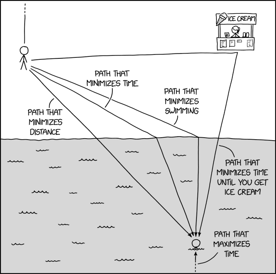
How many ways can you arrange 128 tennis balls?

I found this bit of computational mathematics fascinating. From http://www.joh.cam.ac.uk/how-many-ways-can-you-arrange-128-tennis-balls-researchers-solve-apparently-impossible-problem:

Imagine that you have 128 soft spheres, a bit like tennis balls. You can pack them together in any number of ways. How many different arrangements are possible?

The answer, it turns out, is something like 10²⁵⁰ (1 followed by 250 zeros). The number, also referred to as ten unquadragintilliard, is so huge that it vastly exceeds the total number of particles in the universe.

Far more important than the solution, however, is the fact that the researchers were able to answer the question at all. The method that they came up with can help scientists to calculate something called configurational entropy – a term used to describe how structurally disordered the particles in a physical system are.

Irrational / Everything’s relative

One popular (though maybe apocryphal) story from the history of mathematics involves the discovery of irrational numbers by Pythagoras and his disciples. The following quote is from the book Fermat’s Last Theorem by Simon Singh:

One story claims that a young student by the name of Hippasus was idly toying with the number $\sqrt{2}$ , attempting to find the equivalent fraction. Eventually he came to realize that no such fraction existed, i.e. that $\sqrt{2}$ is an irrational number. Hippasus must have been overjoyed by his discovery, but his master was not. Pythagoras had defined the universe in terms of rational numbers, and the existence of irrational numbers brought his ideal into question. The consequence of Hippasus’ insight should have been a period of discussion and contemplation during which Pythagoras ought to have come to terms with this new source of numbers. However, Pythagoras was unwilling to accept that he was wrong, but at the same time he was unable to destroy Hippasus’ argument by the power of logic. To his eternal shame he sentenced Hippasus to death by drowning.

When I was a boy, the story was told that Pythagoras could not accept irrational (i.e.., cannot be written as the ratio of two integers) numbers because their existence would mean that we live in an irrational (i.e., insane, crazy) world, and so he had the unfortunate discoverer silenced.

When I present this story to my own students, they’re usually incredulous about the story, doubting that someone so smart could act so stupidly (or irrationally). Then I’ll tell them a much more recent story, from less than 100 years ago, about how a scientific principle morphed into a statement of ethics. Einstein’s theories of special relativity and general relativity were developed in the early 1900s; his theory of general relativity explained precession in the orbit of Mercury and predicted the deflection of starlight by the Sun’s gravity, which were both unexplained by Newtonian mechanics.

Writing to a popular audience, Einstein summarized his theory as follows:

The ‘Principle of Relativity’ in its widest sense is contained in the statement: The totality of physical phenomena is of such a character that it gives no basis for the introduction to the concept of “absolute motion”; or, shorter but less precise: There is no absolute motion.

The following sentences from Paul Johnson’s Modern Times summarize the popular reaction to Einstein’s work:

But for most people, to whom Newtonian physics, with their straight lines and right angles, were perfectly comprehensible, relativity never became more than a vague source of unease. It was grasped that absolute time and absolute length had been dethroned; that motion was curvilinear… At the beginning of the 1920s the belief began to circulate, for the first time at a popular level, that there were no longer any absolutes: of time and space, of good and evil, of knowledge, above all of value. Mistakenly, but perhaps inevitably, relativity became confused with relativism.

Indeed, the modern catchphrase “everything’s relative” was spawned shortly after the discovery of special and general relativity, a moral principle that Einstein himself abhorred.

So, after telling the story about Pythagoras and $\sqrt{2}$ , I’ll use this story to hold up a mirror to ourselves, demonstrating that the passage of time has not made us immune from translating mathematical or scientific principles into statements of ethics.

Mathematics that Swings: The Math Behind Golf

From the YouTube description:

Mathematics is everywhere, and the golf course is no exception. Many aspects of the game of golf can be illuminated or improved through mathematical modeling and analysis. We will discuss a few examples, employing mathematics ranging from simple high school algebra to computational techniques at the frontiers of contemporary research.

Interesting calculus problems

Source: http://xkcd.com/135/

Design Zone at Fort Worth Museum of Science and History

If you live in the Dallas-Fort Worth metroplex or are visiting this summer, I highly recommend Design Zone, which is on exhibit at the Fort Worth Museum of Science and History until September 7. I’ve been to a lot of science museums, so I don’t make the following statement lightly: this may well be the most fun and most engaging physics exhibit for children to enjoy that I’ve ever seen. There’s all kinds of things to lift, throw, balance, and blast off so that children have so much fun that they don’t even realize that they’ve learned something.

Here’s the information posted by the museum: http://fwmuseum.org/design-zone

Here’s a short promotional video:

And here’s a longer video describing the exhibit:

Symphonic Equations: Waves and Tubes

This excellent and engaging video describes how sine and cosine functions can be applied to music.

Why Science Teachers Should Not Be Given Playground Duty

Source: https://www.facebook.com/KMPHFOX26/photos/a.211376604011.169435.210413314011/10152781377649012/?type=1&theater

Sphere

Source: http://www.xkcd.com/1248/

Exponential growth and decay (Part 16): Logistic growth model

In this series of posts, I provide a deeper look at common applications of exponential functions that arise in an Algebra II or Precalculus class. In the previous posts in this series, I considered financial applications, radioactive decay, and Newton’s Law of Cooling.

Today, I discuss the logistic growth model, which describes how an infection (like a disease, a rumor, or advertise) spreads in a population. In yesterday’s post, I described an in-class demonstration that engages students while also making the following formula believable:

$A(t) = \displaystyle \frac{Ly_0}{y_0+ (L-y_0)e^{-rt}}$ .

I’d like to discuss some observations about this somewhat complicated function that will make producing its graph easier. The first two observations are within reach of Precalculus students.

1. Let’s figure out the $y-$ intercept:

$A(0) = \displaystyle \frac{Ly_0}{y_0+ (L-y_0)e^{-r \cdot 0}} = \displaystyle \frac{Ly_0}{y_0+ L-y_0} = y_0$ .

In other words, the number $y_0$ represents the initial number of people who have the infection.

2. Let’s figure out the limiting value as $t$ gets large:

$\displaystyle \lim_{t \to \infty} A(t) = \displaystyle \frac{Ly_0}{y_0+ (L-y_0) \cdot 0} = \displaystyle \frac{Ly_0}{y_0} = L$ .

As expected, all $L$ people will get the infection eventually. (Of course, Precalculus students won’t be familiar with the $\displaystyle \lim$ notation, but they should understand that $e^{-rt}$ decays to zero as $t$ gets large.

3. Let’s now figure out the point of inflection. Ordinarily, points of inflection are found by setting the second derivative equal to zero. Though this can be done for the function $A(t)$ above, it would be a somewhat daunting exercise!

The good news is that the points of inflection can be found quite simply using the governing differential equation, which is

$A' = r A [ L - A] = r L A - r A^2$

Let’s take the derivative of both sides, remembering that $r$ and $L$ are constants:

$A'' = r L A' - 2 r A A'$

$A'' = A' (r L - 2 r A)$

So the second derivative is equal to zero when either $A' = 0$ or else $r L - 2 r A = 0$ . The first case corresponds to the trivial cases $A(t) \equiv 0$ and $A(t) \equiv L$ ; these constants are called the equilibrium solutions. The second case is the more interesting one:

$r L - 2 r A = 0$

$r L = 2 r A$

$\displaystyle \frac{L}{2} = A$

This suggests that, as the infection spreads throughout a population, the curve changes concavity at the time that half of the population becomes infected. In other words, the infection spreads fastest throughout the population at the time when half of the population has been infected.

The time at which the point of inflection occurs can be found by setting $A(t) = \displaystyle \frac{L}{2}$ and solving for $t$ :

$\displaystyle \frac{L}{2} = \displaystyle \frac{Ly_0}{y_0+ (L-y_0)e^{-rt}}$ .

$\displaystyle \frac{1}{2} = \displaystyle \frac{y_0}{y_0+ (L-y_0)e^{-rt}}$ .

$y_0 + (L-y_0) e^{-rt} = 2y_0$

$(L-y_0) e^{-rt} = y_0$

$e^{-rt} = \displaystyle \frac{y_0}{L-y_0}$

$-rt = \displaystyle \ln \left( \frac{y_0}{L-y_0} \right)$

$t = \displaystyle - \frac{1}{r} \ln \left( \frac{y_0}{L-y_0} \right)$

This technique for finding the points of inflection directly from the differential equation is possible whenever the differential equation is autonomous, which loosely means that the independent variable does not appear on the right-hand side.

Exponential growth and decay (Part 15): Logistic growth model

Today, I introduce the logistic growth model, which describes how an infection (like a disease, a rumor, or advertise) spreads in a population. For example:

Sources: http://www.xkcd.com/1220/ and http://www.xkcd.com/1235/

In yesterday’s post, I described an in-class demonstration that engages students while also making the following formula believable:

$A(t) = \displaystyle \frac{L}{1 + (L-1)e^{-rt}}$ .

Where does this formula come from? Suppose that a disease is spreading in a population of size $L$ . It stands to reason that the rate at which the disease spreads is proportional to the number of possible contacts between those who have the disease and those who don’t. If $A(t)$ is the number of people who have the disease, then $L-A(t)$ is the number of people who don’t have the disease. Therefore, the product $A(t) [ L - A(t) ]$ is the number of possible contacts between those who have the disease and those who don’t. This leads to the governing differential equation

$A'(t) = c A(t) [ L - A(t) ]$ ,

where $c$ is the constant of proportionality. This is often rewritten by letting $c = \displaystyle \frac{r}{L}$ , or $r = cL$ :

$A'(t) = \displaystyle \frac{r}{L} A(t) [ L - A(t) ]$

$A'(t) = r A(t) \displaystyle \left[1 - \frac{A(t)}{L} \right]$

The good news is that this differential equation can be solved using separation of variables, just like the governing differential equations for continuous compound interest, paying off credit card debt, radioactive decay, and Newton’s Law of Cooling. The bad news is that it’s a lot harder to calculate the required integrals! After all, the right-hand side, after distributing, has a term containing $A^2$ , which makes this differential equation non-linear.

Solving this differential equation is a bit tedious, and I don’t feel particularly obligated to re-invent the wheel since it can be found several places on the Internet. Suffice it to say that integration by partial fractions and some very tricky algebra is necessary to solve for $A(t)$ and obtain the solution above. Among several different sources (which likely use different letters than the ones I’m using here):

Wikipedia: http://en.wikipedia.org/wiki/Logistic_function#In_ecology:_modeling_population_growth

MathWorld: http://mathworld.wolfram.com/LogisticEquation.html