There are two apparently different definitions of a logarithm that appear in the secondary mathematics curriculum:
- From Algebra II and Precalculus: If
 and
and  , then
  is the inverse function of
  .
.
- From Calculus: for
 , we define
  .
.
The connection between these two apparently different ideas begins with the following theorem, which was proven in the few previous posts.
Theorem. Let  . Suppose that
  has the following four properties:


 for all
 is continuous
Then for all  .
.
 At this point, we have provided enough groundwork to make the connection between these two different ways of viewing a logarithm.
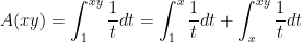
Let’s define the function (for )
 .
.
I’ll illustrate this with the appropriate area under the hyperbola  . (Please forgive the crudeness of this drawing; I’m only using Microsoft Paint.)
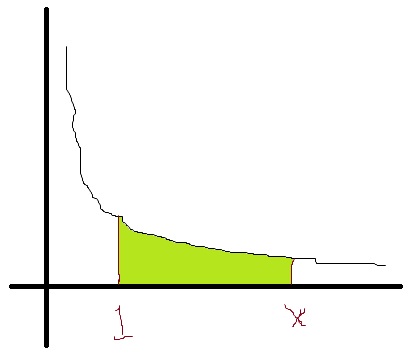 So if
So if  is the right-hand limit, then
  is just the shaded area under the curve.
Often, someone will interject, “Hey, I know how to do that… it’s just the natural logarithm of .” To which I will respond, “Yes, that’s true. But why is it the natural logarithm of ?” I have yet to encounter a student who can immediately answer this question (which, of course, is the whole point of me presenting this in class). In other words, I want my students to realize that, many semesters ago, they pretty much accepted on faith that the above integral is equal to  , but they were never told the reason why. And now — several semesters after completing the calculus sequence — we’re finally going over the reason why.
To start, I’ll say, “OK,  is defined as an integral. That means that it must have…” Someone will usually volunteer, “A derivative.” I’ll respond, “That’s right. The Fundamental Theorem of Calculus says that this function is differentiable. So, if something is differentiable, then it also must be…” Someone will usually volunteer, “Continuous.” My response: “That’s right. So must be continuous. So that’s Property 4: this function is continuous.” I’ll continue: “Let’s see if we can get the other properties.”
I’ll next move to Property 1, as it’s the next easiest. I’ll ask the class, “Can you prove to me that  ?” After a moment of thought, someone will notice that
 .
.
must be equal to  since the left and right endpoints of the integral are the same.
Then I’ll skip over to Property 3, which requires a little more thought. To begin, we can write
 .
.
Before proceeding, I’ll ask my class why the above line has to be true. After a couple moments, someone will volunteer something like “The area from  to plus the area from to
  has to be equal to the area from to .”
I’ll then say something like, “We can simplify one of the integrals on the right-hand side right away. Which one?” Students quickly see that the first integral on the right,  , is of course equal to . So then I’ll ask, “So what do I want the last integral to be equal to?” Students look back at Property 3 and answer, “That should be
  .
.
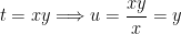
So, if we can show the final integral is equal to , we have established Property 3. To this end, I will perform a somewhat unusual looking  substitution:

In this formula, I encourage my students to think of  as the old variable of integration,
  as the new variable of integration, and as an unknown number that is constant. So I’ll say parenthetically, “If
  , how do we find
  ?” Students of course answer, “ must be
  .” So I’ll follow up: “If
  , how do we find ?” Students get the idea:

So to complete the substitution, we must adjust the limits of integration. For the lower limit,

For the upper limit,
So we can now complete the substitution of the second integral:
.
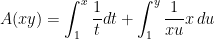 .
.
 .
.
Students recognize that, except for the variable of integration, the last integral is just , which leads to the punch line

In other words, we have established that the function satisfies Property 3.
So the only property left is Property 2. To that end, let’s define the number  so that the area in green above is equal to 1. There’s no other way to describe this number…. we just increase far enough along the
  axis until the area under the hyperbola is equal to 1. Wherever this happens, that’s the number that we’ll call . So, by definition,
  .
.
Therefore, by the above theorem, we conclude that  , written more simply as .
To summarize: using the above theorem, we are able to establish that the integral  has all of the properties of a logarithm and therefore must be a logarithmic function. The only catch is that we had to define to be the base of this logarithm through an unusual definition concerning the area under a hyperbola.
Of course, this is not the “standard” definition of that is usually encountered in a Precalculus class. More on these different definitions in a future series of posts.
One more pedagogical note: My experience is that I can cover the content of the first 7 posts of this series in a single 50-minute lecture and still keep my students’ attention. Naturally, I’ll recapitulate the highlights of this logical development at the start of the next lecture by way of review, as this is an awful lot to absorb at once.
dollars are invested at interest rate
for
.
from
to
is equal to


 At this point in the exposition, I have justified the formula


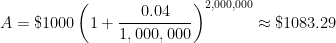

 a few times and see if a pattern can be developed. However, my observation is that college students have no memory of being taught how the compound interest formula
 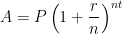 can be seen as a natural consequence of the simple interest formula. In other words, they’d just use the compound interest formula without having any conceptual understanding of where the formula came from.
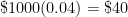 .
. .
. .
. .
. .
. .
. .
. .
. .
. .
. .
.
 .
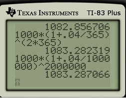
. is indeed equal to
  .
. .
. .
. .
. .
. .
. . The
. The  comes from dividing the 4% into four parts. The 8 comes from the number of compounding periods over 2 years.
 . The above argument justifies the formula; the actual proof of the formula is very similar to the above numerical examples, and so I don’t use class time to formally prove it.


 is just a constant, we conclude
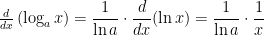


 . To this end, let’s apply implicit differentiation to this last equation:


 and
and  on their own after class.
 in Theorem 3. Alternatively, repeat the above argument for the inverse functions
  and
and  , thus proving that
 , where


 . And this single case is simply handled through Property 1:
 . There is a natural way to approximate


 .
.
 .
.

 be a sequence of rational numbers that converges to
 .
. , this means that
 .
. .
.

 is a sequence that converges to
  . So, if we replace
  by
by  and
and  , we conclude that


 , even if


 , a negative rational number.
 ?” This leads to the proof of Case 3. I’ve found that it’s helpful to walk through this proof line by line in step with the case of
  , so that students can see how the steps of this more abstract proof correspond to the concrete example of
  .
. . Then


![2 = f(a^2) = f \left( \left[a^{2/3} \right]^3 \right)](https://s0.wp.com/latex.php?latex=2+%3D+f%28a%5E2%29+%3D+f+%5Cleft%28+%5Cleft%5Ba%5E%7B2%2F3%7D+%5Cright%5D%5E3+%5Cright%29&bg=ffffff&fg=000000&s=0&c=20201002)


 term?” The obvious correct answer:
 .
. ?” This leads to the proof of Case 2. I’ve found that it’s helpful to walk through this proof line by line in step with the case of
  , so that students can see how the steps of this more abstract proof correspond to the concrete example of
  .
. where
where  . Then
![m = f \left( \left[ a^{m/n} \right]^n \right)](https://s0.wp.com/latex.php?latex=m+%3D+f+%5Cleft%28+%5Cleft%5B+a%5E%7Bm%2Fn%7D+%5Cright%5D%5En+%5Cright%29&bg=ffffff&fg=000000&s=0&c=20201002)


 ?” Someone will usually suggest
  , and so I’ll write this as the next step:


 .
. , so that students can see how the steps of this more abstract proof correspond to the concrete example of
  .
.


 and
and  , then
  is the inverse function of
  .
. for all
  . That’s almost correct, and so I’ll ask if Property 2 is satisfied by this function. After a couple more moments of thought, someone will volunteer the correct answer,
  defined by
  must be equal to
  .
.