In this series, I’m discussing how ideas from calculus and precalculus (with a touch of differential equations) can predict the precession in Mercury’s orbit and thus confirm Einstein’s theory of general relativity. The origins of this series came from a class project that I assigned to my Differential Equations students maybe 20 years ago.
We previously showed that if the motion of a planet around the Sun is expressed in polar coordinates 

where 


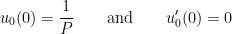
We will also impose the initial condition that the planet is at perihelion (i.e., is closest to the sun), at a distance of 


the second equation arises since
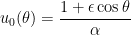
In previous posts, we showed that the solution of this initial-value problem is
where 

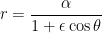
so that, as shown earlier in this series, the orbit is an ellipse with eccentricity 

At long last, we’re now ready to see what happens under general relativity. According to the theory of general relativity, the governing differential equation for the orbit of a planet should be changed ever so slightly to
![u''(\theta) + u(\theta) = \displaystyle \frac{Gm^2 M}{\ell^2} + \frac{3GM}{c^2} [u(\theta)]^2](https://s0.wp.com/latex.php?latex=u%27%27%28%5Ctheta%29+%2B+u%28%5Ctheta%29+%3D+%5Cdisplaystyle+%5Cfrac%7BGm%5E2+M%7D%7B%5Cell%5E2%7D+%2B+%5Cfrac%7B3GM%7D%7Bc%5E2%7D+%5Bu%28%5Ctheta%29%5D%5E2&bg=ffffff&fg=000000&s=0&c=20201002)
where a second term was added to the right-hand side. (I will make no attempt here to justify the physics for this second term.) In this second term, 

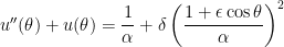
![u''(\theta) + u(\theta) = \displaystyle \frac{1}{\alpha} + \delta [u(\theta)]^2](https://s0.wp.com/latex.php?latex=u%27%27%28%5Ctheta%29+%2B+u%28%5Ctheta%29+%3D+%5Cdisplaystyle+%5Cfrac%7B1%7D%7B%5Calpha%7D+%2B+%5Cdelta+%5Bu%28%5Ctheta%29%5D%5E2&bg=ffffff&fg=000000&s=0&c=20201002)
Finding an exact solution of this new differential equation is hopeless. While the previous differential equation was linear with constant coefficients, this new differential is decidedly nonlinear because of the new term ![[u(\theta)]^2](https://s0.wp.com/latex.php?latex=%5Bu%28%5Ctheta%29%5D%5E2&bg=ffffff&fg=000000&s=0&c=20201002)
So, instead of attempting to find an exact solution, we will use the method of successive approximations, mentioned earlier in this series, to find an approximate solution that is very, very close to the exact solution. Since 
will be approximately equal to the solution of the “real” differential equation under general relativity. We have already shown that the solution of this simpler differential equation is
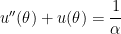
Therefore, the method of successive approximations suggests that a better approximation to the true orbit will be the solution of
![u''(\theta) + u(\theta) = \displaystyle \frac{1}{\alpha} + \delta [u_0(\theta)]^2](https://s0.wp.com/latex.php?latex=u%27%27%28%5Ctheta%29+%2B+u%28%5Ctheta%29+%3D+%5Cdisplaystyle+%5Cfrac%7B1%7D%7B%5Calpha%7D+%2B+%5Cdelta+%5Bu_0%28%5Ctheta%29%5D%5E2&bg=ffffff&fg=000000&s=0&c=20201002)
or
While significantly messier than the differential equation under Newtonian mechanics, this is now a linear differential equation that can be solved using standard techniques from differential equations. In the next few posts, we will solve this new differential equation, thus finding the predicted orbit of a planet under general relativity.
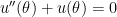
 , with the Sun at the origin, then under Newtonian mechanics (i.e., without general relativity) the motion of the planet follows the differential equation
  and
and  is a certain constant. We will also impose the initial condition that the planet is at perihelion (i.e., is closest to the sun), at a distance of
 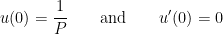 ;
; .
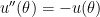
. , which clearly has the two imaginary roots
  . Therefore, two linearly independent solutions of the associated homogeneous equation are
  and
and  .
. , but complex numbers provide a way of solving the differential equations that model multiple problems in statics and dynamics.)
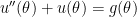
 ,
, ,
, ,
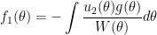
, is the Wronskian of
  and
and  , defined by the determinant
 .
.
 and
and  essentially disappear.
 , the integrals for
  ,
, for the constant of integration instead of the usual
  . Second,
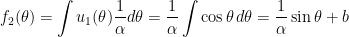 ,
, for the constant of integration. Therefore, by variation of parameters, the general solution of the nonhomogeneous differential equation is
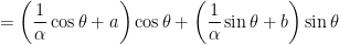
 .
. and
and  . This is require using the initial conditions
  and
and  . From the first initial condition,


 .
.
 ,
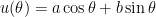
, , we see that the planet’s orbit satisfies
 .
. is not a solution of the characteristic equation, this leads to trying something of the form
  as a solution, where
  is a soon-to-be-determined constant. (Guessing this form of
  is a standard technique from differential equations; later in this series, I’ll give some justification for this guess.)
 and
and  . Substituting, we find


 is a particular solution of the nonhomogeneous differential equation.
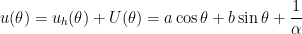 .
.
 .
. and
and  .
. and
and  work. Once that conceptual barrier is broken, they’ll usually produce the solutions
  and
and  .
. also solves the associated homogeneous differential equation.
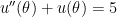 . Can you think of an easy function that’s a solution?
 is a constant function, then clearly
  and
and  , so that
  works.
 is a solution of
  is a solution of
  will work.
 :
: and then substitute