Confirming Einstein’s Theory of General Relativity With Calculus, Part 2a: Graphically Exploring Precession

In this series, I’m discussing how ideas from calculus and precalculus (with a touch of differential equations) can predict the precession in Mercury’s orbit and thus confirm Einstein’s theory of general relativity. The origins of this series came from a class project that I assigned to my Differential Equations students maybe 20 years ago.

But what is precession? To explore this concept, let’s explore the graph of

for various values of , , and using Desmos. (Note that, in this context, the number does not mean Euler’s constant . The reason for choosing the letter for this parameter will become clear shortly.) Naturally, this demonstration could also be done with other tools like a graphing calculator.

I suggest beginning by setting and and altering the value of . This is the easiest behavior to explain. From the equation, is directly proportional to the distance from the origin . So, not surprisingly, increasing produces a larger graph, and decreasing produces a smaller graph.

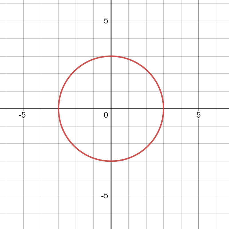
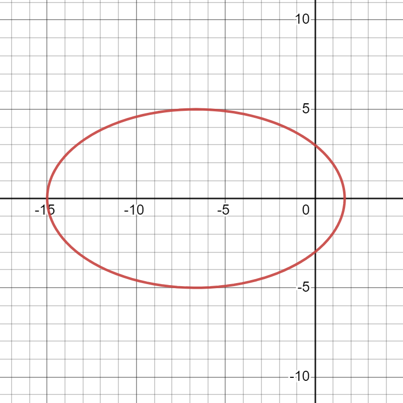
Second, I suggest setting and but altering the value of . Starting at , the graph is a circle. This makes complete sense: if , then the equation simply becomes , so the distance from the origin is the same for all angles. However, as increases, the original circle becomes more and more stretched out. We will prove this analytically in a later post, but it turns out that, for , the graph is an ellipse, and the origin is one of the foci of the ellipse. The number is called the eccentricity of the ellipse (hence the letter ).

Again, if the value of is fixed but varies, the graph becomes either larger or smaller as becomes larger or smaller.

We notice that if and , then the denominator of

varies between and . In particular, the denominator is always positive. Therefore, the value of is least positive — the graph is closest to the origin — when the denominator is greatest. This happens when is a multiple of . So, for example, when , then is as close as the graph gets to the origin. Let’s call this closest distance ; in the context of a planet’s orbit around the sun, this represent perihelion. Then we have .

When , the graph switches from an ellipse to a parabola, where the origin is the focus of the parabola. For , the graph becomes a hyperbola. However, since we’re mostly going to be concerned with stable planetary orbits in this series, we won’t dwell too much on the case .

Third, I suggest setting , , and then alter the value of . For , the graph is simply a single ellipse. However, by changing the value of , the graph changes into a spiral.

In the above figure, the spiral stopped “spiraling” because I had asked Desmos only to show the graph between . If I had changed the upper bound to something larger than , the spiral would continue.

The precession in the spiral is defined to be the angular offset between each loop of the spiral. Clearly, this is a function of . To find this function, we again examine the function

Once again, if , then the denominator varies between and . In particular, the denominator is always positive. Therefore, the value of is least positive when the denominator is greatest, and the denominator is greatest when is a multiple of . So, for example, when , then is as close as the graph gets to the origin.

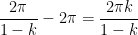
When does the graph return to its closest point to the origin next? This would occur when , or . If , then the angle of closest approach to the origin would , and the graph simply cycles over itself. However, if , then this angle will be larger than , thus producing a spiral. Indeed, the amount of precession would be equal to

.

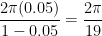
In the picture above, . Therefore, the amount of precession would be radians . Therefore, after 19 “leafs” of the spiral, the graph would begin to cycle on top of itself.