In this series, I’m discussing how ideas from calculus and precalculus (with a touch of differential equations) can predict the precession in Mercury’s orbit and thus confirm Einstein’s theory of general relativity. The origins of this series came from a class project that I assigned to my Differential Equations students maybe 20 years ago.
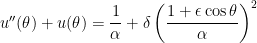
We have shown that the motion of a planet around the Sun, expressed in polar coordinates  with the Sun at the origin, under general relativity follows the initial-value problem
 ,
,
 ,
,
 ,
,
where  ,
,  ,
,  ,
,  is the gravitational constant of the universe,
  is the mass of the planet,
  is the mass of the Sun,
  is the constant angular momentum of the planet,
  is the speed of light, and
  is the smallest distance of the planet from the Sun during its orbit (i.e., at perihelion).
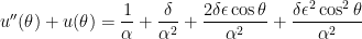
We now take the perspective of a student who is taking a first-semester course in differential equations. There are two standard techniques for solving a second-order non-homogeneous differential equations with constant coefficients. One of these is the method of constant coefficients. To use this technique, we first expand the right-hand side of the differential equation and then apply a power-reduction trigonometric identity:
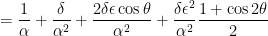
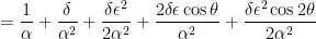
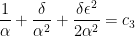
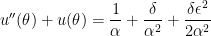
This is now in the form for using the method of undetermined coefficients. However, in this series, I’d like to take some time to explain why this technique actually works. To begin, we look at a simplified differential equation using only the first three terms on the right-hand side:
 .
.
Let 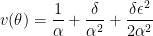 . Since
  is a constant, this function satisfies the simple differential equation
  . Since
  , we can substitute:


(We could have more easily said, “Take the derivative of both sides,” but we’ll be using a more complicated form of this technique in future posts.) The characteristic equation of this differential equation is  . Factoring, we obtain
  , so that the three roots are
  and
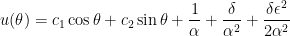
and  . Therefore, the general solution of this differential equation is
 .
.
Notice that this matches the outcome of blindly using the method of undetermined coefficients without conceptually understanding why this technique works.
The constants  and
and  are determined by the initial conditions. To find
  , we observe

 .
.
Therefore, the general solution of this simplified differential equation is
 .
.
Furthermore, setting  , we see that

is a particular solution to the differential equation
 .
.
In the next couple of posts, we find the particular solutions associated with the other terms on the right-hand side.
are chosen at random (uniformly) from the interior of a unit circle. What is the probability that the circle whose diameter is segment
lies entirely in the interior of the unit circle?


![= \displaystyle \frac{2}{3} \left[ u^{3/2} \right]_0^1](https://s0.wp.com/latex.php?latex=%3D+%5Cdisplaystyle+%5Cfrac%7B2%7D%7B3%7D+%5Cleft%5B++u%5E%7B3%2F2%7D+%5Cright%5D_0%5E1&bg=ffffff&fg=000000&s=0&c=20201002)
![=\displaystyle \frac{2}{3}\left[ (1)^{3/2} - (0)^{3/2} \right]](https://s0.wp.com/latex.php?latex=%3D%5Cdisplaystyle++%5Cfrac%7B2%7D%7B3%7D%5Cleft%5B+%281%29%5E%7B3%2F2%7D+-+%280%29%5E%7B3%2F2%7D+%5Cright%5D&bg=ffffff&fg=000000&s=0&c=20201002)


 .
. ;
; and
and  to write
  and
and  as double sums and then interchanging the order of summation.
![g'(x) = \displaystyle \sum_{n=0}^\infty \left( [\sin x]' - [x]' + \left[\frac{x^3}{3!}\right]' - \left[\frac{x^5}{5!}\right]' \dots + \left[(-1)^{n-1} \frac{x^{2n+1}}{(2n+1)!}\right]' \right)](https://s0.wp.com/latex.php?latex=g%27%28x%29+%3D+%5Cdisplaystyle+%5Csum_%7Bn%3D0%7D%5E%5Cinfty+%5Cleft%28+%5B%5Csin+x%5D%27+-+%5Bx%5D%27+%2B+%5Cleft%5B%5Cfrac%7Bx%5E3%7D%7B3%21%7D%5Cright%5D%27+-+%5Cleft%5B%5Cfrac%7Bx%5E5%7D%7B5%21%7D%5Cright%5D%27+%5Cdots+%2B+%5Cleft%5B%28-1%29%5E%7Bn-1%7D+%5Cfrac%7Bx%5E%7B2n%2B1%7D%7D%7B%282n%2B1%29%21%7D%5Cright%5D%27+%5Cright%29&bg=ffffff&fg=000000&s=0&c=20201002)


 .
. term. I begin by separating the
  term from the sum, so that a sum from
  to
to  remains:
 .
.![f'(x) = (\cos x - 1)' + \displaystyle \sum_{n=1}^\infty \left( [\cos x - 1]' + \left[ \frac{x^2}{2!} \right]' - \left[ \frac{x^4}{4!} \right]' \dots + \left[ (-1)^{n-1} \frac{x^{2n}}{(2n)!} \right]' \right)](https://s0.wp.com/latex.php?latex=f%27%28x%29+%3D+%28%5Ccos+x+-+1%29%27+%2B+%5Cdisplaystyle+%5Csum_%7Bn%3D1%7D%5E%5Cinfty+%5Cleft%28+%5B%5Ccos+x+-+1%5D%27+%2B+%5Cleft%5B+%5Cfrac%7Bx%5E2%7D%7B2%21%7D+%5Cright%5D%27+-+%5Cleft%5B+%5Cfrac%7Bx%5E4%7D%7B4%21%7D+%5Cright%5D%27+%5Cdots+%2B+%5Cleft%5B+%28-1%29%5E%7Bn-1%7D+%5Cfrac%7Bx%5E%7B2n%7D%7D%7B%282n%29%21%7D+%5Cright%5D%27+%5Cright%29&bg=ffffff&fg=000000&s=0&c=20201002)


 .
. , so that
  and
and  varies from
  to
to  .
.


 term, this sum is exactly the definition of

 .
. and
and  . Differentiating
  a second time, we obtain
 .
. . Substituting, we see that
![[Ax \cos x + B x \sin x]'' + A x \cos x + Bx \sin x = -\cos x](https://s0.wp.com/latex.php?latex=%5BAx+%5Ccos+x+%2B+B+x+%5Csin+x%5D%27%27+%2B+A+x+%5Ccos+x+%2B+Bx+%5Csin+x+%3D+-%5Ccos+x&bg=ffffff&fg=000000&s=0&c=20201002)


 and
and  which then lead to the particular solution
 , we conclude that
 ,
, . As it turns out, it is straightforward to compute
  and
and  , so we will choose
  for the initial conditions. We observe that
  are both clearly equal to 0, so that
  as well.
  clearly imples that
  :
:


 .
. , and so

 .
. by writing the series as a double sum and then reversing the order of summation. We proceed with very similar logic to evaluate


 .
. in the summand; however, the denominator is
 ,
, . Hypothetically, I could cancel as follows:
 ,
, and then distribute and split into two different sums:

![= \displaystyle \frac{1}{2} \sum_{k=1}^\infty \left[ (-1)^k (2k+1) \frac{x^{2k+1}}{(2k+1)!} - (-1)^k \cdot 1 \frac{x^{2k+1}}{(2k+1)!} \right]](https://s0.wp.com/latex.php?latex=%3D+%5Cdisplaystyle+%5Cfrac%7B1%7D%7B2%7D+%5Csum_%7Bk%3D1%7D%5E%5Cinfty+%5Cleft%5B+%28-1%29%5Ek+%282k%2B1%29+%5Cfrac%7Bx%5E%7B2k%2B1%7D%7D%7B%282k%2B1%29%21%7D+-+%28-1%29%5Ek+%5Ccdot+1+%5Cfrac%7Bx%5E%7B2k%2B1%7D%7D%7B%282k%2B1%29%21%7D+%5Cright%5D&bg=ffffff&fg=000000&s=0&c=20201002)


 .
. from the first sum. In this way, the two sums are the Taylor series expansions of


 .
.
 .
. .
. ), we see
 .
. cancels:

 and a power of
  .
.
 .
.


 increases, so that the answer should have the form
  or
or  , where
  is an increasing function. I also notice that the graph is symmetric about the origin, so that the function is even. I also notice that the graph passes through the origin.
 , which is satisfies all of the above criteria.
 .
.
 is the answer, of course, but it’s certainly a good indicator.
 and
and 
 near
near  (or, more generally, their Taylor series approximations)
 substitution
 ,
,
 ,
, , and so these can be expected to be small adjustments to an elliptical orbit.

 and
and  . By contrast, the term
 , the planet’s orbit may be accurately described by only including this last perturbation:
 .
. ,
,
 . Differentiating, we find
  ,
,  , etc. Therefore, the differential equation becomes


 can never be equal to
  . Therefore, solving the differential equation reduces to finding the roots of this polynomial, which can be done using standard techniques from Precalculus.
 . The characteristic equation is
  , which has roots
  . Therefore, two solutions to the differential equation are
  and
and  , so that the general solution is
 .
. , so that


 .
. . To find the roots of the characteristic equation, we factor:


 .
. , and
, and  , so that the general solution is
 .
. .
. ,
, .
. .
. .
. . Then
  . Also,
  . Substituting, we find


 .
. can be found by substituting back into the original differential equation:

 and
and  . Therefore, the solution of the simplified differential equation is
 .
. , we see that
